Dataset Sufficiency Analysis for Classification Tutorial
Problem Statement
For machine learning tasks, often we would like to evaluate the performance of a model on a small, preliminary dataset. In situations where data collection is expensive, we would like to extrapolate hypothetical performance out to a larger dataset.
DAML has introduced a method projecting performance via sufficiency curves.
When to use
The Sufficiency class should be used when you would like to extrapolate hypothetical performance. For example, if you have a small dataset, and would like to know if it is worthwhile to collect more data.
What you will need
A particular model architecture.
Metric(s) that we would like to evaluate.
A dataset of interest.
Setting up
Let’s import the required libraries needed to set up a minimal working example
import random
from typing import Dict, Sequence, cast

import matplotlib.pyplot as plt
import numpy as np
import torch
import torch.nn as nn
import torch.nn.functional as F
import torch.optim as optim
import torchmetrics
import torchvision.datasets as datasets
import torchvision.transforms.v2 as v2
from torch.utils.data import DataLoader, Dataset, Subset

from daml.workflows import Sufficiency

np.random.seed(0)
np.set_printoptions(formatter={"float": lambda x: f"{x:0.4f}"})
torch.manual_seed(0)
torch.set_float32_matmul_precision("high")
device = "cuda" if torch.cuda.is_available() else "cpu"
torch._dynamo.config.suppress_errors = True

random.seed(0)
torch.use_deterministic_algorithms(True)
os.environ["CUBLAS_WORKSPACE_CONFIG"] = ":4096:8"
Load data and define functions
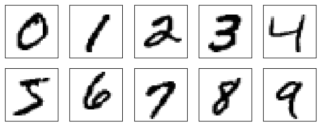
Load the MNIST data and create the training and test datasets.
# Download the mnist dataset and preview the images
to_tensor = v2.Compose([v2.ToImage(), v2.ToDtype(torch.float32, scale=True)])
train_ds = datasets.MNIST("./data", train=True, download=True, transform=to_tensor)
test_ds = datasets.MNIST("./data", train=False, download=True, transform=to_tensor)
fig = plt.figure(figsize=(8, 3))

for lbl in range(10):
    i = (train_ds.targets == lbl).nonzero()[0][0]
    img = train_ds.data[i]
    ax = fig.add_subplot(2, 5, lbl + 1)
    ax.xaxis.set_visible(False)
    ax.yaxis.set_visible(False)
    ax.imshow(img, cmap="gray_r")
For the purposes of this example, we will use subsets of the training (2000) and test (500) data.
# Take a subset of 2000 training images and 500 test images
train_ds = Subset(train_ds, range(2000))
test_ds = Subset(test_ds, range(500))
Next, we define the network architecture we will be using.
# Define our network architecture
class Net(nn.Module):
    def __init__(self):
        super().__init__()
        self.conv1 = nn.Conv2d(1, 6, 5)
        self.conv2 = nn.Conv2d(6, 16, 5)
        self.fc1 = nn.Linear(6400, 120)
        self.fc2 = nn.Linear(120, 84)
        self.fc3 = nn.Linear(84, 10)

    def forward(self, x):
        x = F.relu(self.conv1(x))
        x = F.relu(self.conv2(x))
        x = torch.flatten(x, 1)  # flatten all dimensions except batch
        x = F.relu(self.fc1(x))
        x = F.relu(self.fc2(x))
        x = self.fc3(x)
        return x


# Compile the model
model = torch.compile(Net().to(device))

# Type cast the model back to Net as torch.compile returns a Unknown
# Nothing internally changes from the cast; we are simply signaling the type
model = cast(Net, model)
Finally, we define our custom training and evaluation functions. Sufficiency requires that the evaluation function returns a dictionary of the results.
def custom_train(model: nn.Module, dataset: Dataset, indices: Sequence[int]):
    # Defined only for this testing scenario
    criterion = torch.nn.CrossEntropyLoss().to(device)
    optimizer = optim.SGD(model.parameters(), lr=0.01, momentum=0.9)
    epochs = 10

    # Define the dataloader for training
    dataloader = DataLoader(Subset(dataset, indices), batch_size=16)

    for epoch in range(epochs):
        for batch in dataloader:
            # Load data/images to device
            X = torch.Tensor(batch[0]).to(device)
            # Load targets/labels to device
            y = torch.Tensor(batch[1]).to(device)
            # Zero out gradients
            optimizer.zero_grad()
            # Forward propagation
            outputs = model(X)
            # Compute loss
            loss = criterion(outputs, y)
            # Back prop
            loss.backward()
            # Update weights/parameters
            optimizer.step()
def custom_eval(model: nn.Module, dataset: Dataset) -> Dict[str, float]:
    metric = torchmetrics.Accuracy(task="multiclass", num_classes=10).to(device)
    result = 0

    # Set model layers into evaluation mode
    model.eval()
    dataloader = DataLoader(dataset, batch_size=16)
    # Tell PyTorch to not track gradients, greatly speeds up processing
    with torch.no_grad():
        for batch in dataloader:
            # Load data/images to device
            X = torch.Tensor(batch[0]).to(device)
            # Load targets/labels to device
            y = torch.Tensor(batch[1]).to(device)
            preds = model(X)
            metric.update(preds, y)
        result = metric.compute().cpu()
    return {"Accuracy": result}
Initialize sufficiency metric
Attach the custom training and evaluation functions to the Sufficiency metric and define the number of models to train in parallel (stability), as well as the number of steps along the learning curve to evaluate.
# Instantiate sufficiency metric
suff = Sufficiency(
    model=model,
    train_ds=train_ds,
    test_ds=test_ds,
    train_fn=custom_train,
    eval_fn=custom_eval,
    runs=5,
    substeps=10,
)
Evaluate Sufficiency
Now we can evaluate the metric to train the models and produce the learning curve.
# Train & test model
output = suff.evaluate()
# Print out sufficiency output in a table format
from tabulate import tabulate

formatted = {k: v for k, v in output.items() if k != "_CURVE_PARAMS_"}
print(tabulate(formatted, headers=list(formatted.keys()), tablefmt="pretty"))
+---------+---------------------+
| _STEPS_ |      Accuracy       |
+---------+---------------------+
|   20    | 0.1184000015258789  |
|   33    | 0.25880000591278074 |
|   55    | 0.5140000343322754  |
|   92    | 0.6484000205993652  |
|   154   | 0.7492000102996826  |
|   258   | 0.8159999847412109  |
|   430   | 0.8535999298095703  |
|   718   | 0.8831999778747559  |
|  1198   | 0.9128000259399414  |
|  2000   | 0.9300000190734863  |
+---------+---------------------+
# Print out projected output values
projection = Sufficiency.project(output, [1000, 2000, 4000])
print(tabulate(projection, list(projection.keys()), tablefmt="pretty"))
+---------+--------------------+
| _STEPS_ |      Accuracy      |
+---------+--------------------+
|  1000   | 0.9093243309771407 |
|  2000   | 0.9380920475826995 |
|  4000   | 0.9569461546973748 |
+---------+--------------------+
# Plot the output using the convenience function
_ = Sufficiency.plot(output)
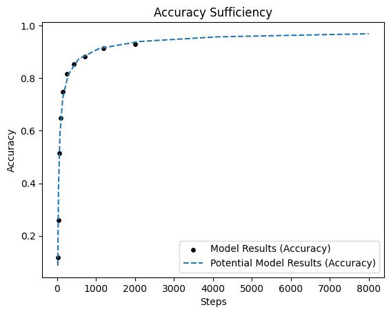
Results
Using this learning curve, we can project performance under much larger datasets (with the same model).
Predicting sample requirements
We can also predict the amount of training samples required to achieve a desired accuracy.
Let’s say we wanted to see how many samples are needed to hit 90%, 95% and 99% accuracy given the learning curve.
# Initialize the array of desired accuracies
desired_accuracies = np.array([0.90, 0.95, 0.99])

# Evaluate the learning curve to infer the needed amount of training data
samples_needed = Sufficiency.inv_project({"Accuracy": desired_accuracies}, output)
# Print the amount of needed data needed to achieve the accuracies of interest
for i, accuracy in enumerate(desired_accuracies):
    print(f"To achieve {accuracy*100}% accuracy, {samples_needed['Accuracy'][i]} training samples are needed.")
To achieve 90.0% accuracy, 841 training samples are needed.
To achieve 95.0% accuracy, 2992 training samples are needed.
To achieve 99.0% accuracy, 261728 training samples are needed.
The projection shows that given the current model, hitting an accuracy of 99% is improbable.