Coverage

Problem Statement

For most computer vision tasks like image classification and object detection, we often have a lot of images, but certain subsets of the images can be undersampled, such as label, style within a label, etc. A way to detect this regional sparsity is through coverage analysis.

To help with this, DataEval has introduced a Coverage class ( Coverage ), that provides a user with example images which have few similar instances within the provided dataset.

When to use

The Coverage class should be used when you have lots of images, but only a small fraction from certain regimes/labels.

What you will need

1. Image classification dataset.

2. Autoencoder trained on image classification dataset for dimension reduction (e.g. through the AETrainer class).

3. A python environment with the following packages installed:

   • dataeval[torch] or dataeval[all]

   • torchvision

   • tabulate

Setting up

Let’s import the required libraries needed to set up a minimal working example

import math

import matplotlib.pyplot as plt  # type: ignore
import numpy as np
import torch
import torch.nn as nn
import torchvision as tv
import torchvision.transforms as transforms
from sklearn.manifold import TSNE  # type: ignore

from dataeval.metrics import coverage

Load the data

We will use the MNIST dataset from torchvision for this tutorial on coverage.

# We train a 10-d autoencoder on MNIST data for 1000 epochs with batch size 128
num_epochs = 1000
batch_size = 128

# Set seeds
torch.manual_seed(14)

# MNIST with mean 0 unit variance
transform = transforms.Compose([transforms.ToTensor(), transforms.Normalize((0.1307,), (0.3081,))])
trainset = tv.datasets.MNIST(root="./data", train=True, download=True, transform=transform)
trainset = torch.utils.data.Subset(trainset, range(2000))
dataloader = torch.utils.data.DataLoader(trainset, batch_size=batch_size, shuffle=True, num_workers=4)

In this tutorial, we will use an autoencoder to reduce the dimension of the MNIST images.

# Define model architecture
class Autoencoder(nn.Module):
    def __init__(self):
        super().__init__()
        self.encoder = nn.Sequential(
            # 28 x 28
            nn.Conv2d(1, 4, kernel_size=5),
            # 4 x 24 x 24
            nn.ReLU(True),
            nn.Conv2d(4, 8, kernel_size=5),
            nn.ReLU(True),
            # 8 x 20 x 20 = 3200
            nn.Flatten(),
            nn.Linear(3200, 10),
            # 10
            nn.Sigmoid(),
        )
        self.decoder = nn.Sequential(
            # 10
            nn.Linear(10, 400),
            # 400
            nn.ReLU(True),
            nn.Linear(400, 4000),
            # 4000
            nn.ReLU(True),
            nn.Unflatten(1, (10, 20, 20)),
            # 10 x 20 x 20
            nn.ConvTranspose2d(10, 10, kernel_size=5),
            # 24 x 24
            nn.ConvTranspose2d(10, 1, kernel_size=5),
            # 28 x 28
            nn.Sigmoid(),
        )

    def forward(self, x):
        x = self.encoder(x)
        x = self.decoder(x)
        return x

    def encode(self, x):
        x = self.encoder(x)
        return x

For computational reasons, we will simply load the trained autoencoder. See the how-to How to create image embeddings with an autoencoder for more information on how to train an autoencoder.

sd = torch.load("models/ae")
model = Autoencoder()
model.load_state_dict(sd)

<All keys matched successfully>

# Get images to predict on and predict
pred = [trainset[i][0] for i in range(2000)]
label = np.array([trainset[i][1] for i in range(2000)])
mod_preds = model.encode(torch.stack(pred)).detach().numpy()

To visualize the encodings, we will use TSNE on them to view separation.

# Visualize 10d as 2d with TSNE
tsne = TSNE(n_components=2)
red_dim = tsne.fit_transform(mod_preds)

# Plot results with color being label
fig, ax = plt.subplots()
scatter = ax.scatter(
    x=red_dim[:, 0],
    y=red_dim[:, 1],
    c=label,
    label=label,
)
ax.legend(*scatter.legend_elements(), loc="upper right", ncols=2)
plt.show()

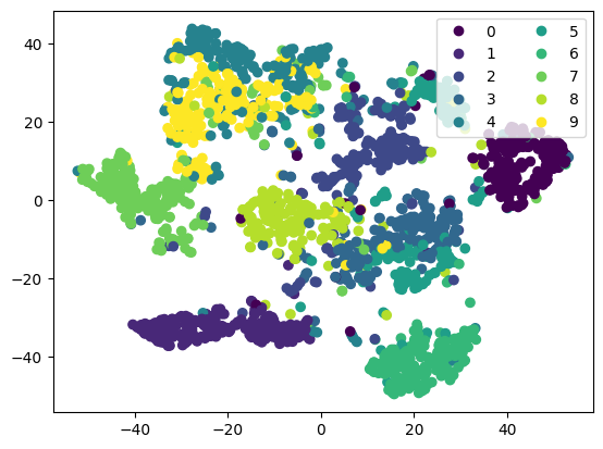
Some good separation, but you can see a few images in the “gaps”. This could be an artifact of dimension reduction, or suggest that we have poor coverage for some covariates.

# Way to calculate data-agnostic radius (probably don't want to do this)
k = 20
n = 2000
d = 10
rho = (1 / math.sqrt(math.pi)) * ((4 * 20 * math.gamma(d / 2 + 1)) / (n)) ** (1 / d)

# Way to calculate data-adaptive radius (most extreme 1% are uncovered)
percent = 0.01
cutoff = int(n * percent)

# Use data adaptive cutoff
cvrg = coverage(mod_preds, radius_type="adaptive")

# Plot the least covered 0.5%
f, axs = plt.subplots(4, 4)
axs = axs.flatten()
for count, i in enumerate(axs):
    i.imshow(np.squeeze(pred[cvrg.indices[count]].numpy()), cmap="gray")

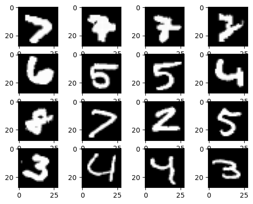
The Coverage tool identified that in this set of 2000 images, there is potential under-coverage when it comes to wonky/ crossed 7s.
Other digits have some undercovered instances, but could be they are just outliers.
More investigation into outlier status is needed, see How to identify outliers and/or anomalies in a dataset for more info.