Coverage

Problem Statement

For most computer vision tasks like image classification and object detection, we often have a lot of images, but certain subsets of the images can be undersampled, such as label, style within a label, etc. A way to detect this regional sparsity is through coverage analysis.

To help with this, DataEval has introduced a Coverage class ( Coverage ), that provides a user with example images which have few similar instances within the provided dataset.

When to use

The Coverage class should be used when you have lots of images, but only a small fraction from certain regimes/labels.

What you will need

1. Image classification dataset.

2. Autoencoder trained on image classification dataset for dimension reduction (e.g. through the AETrainer class).

3. A python environment with the following packages installed:

   • dataeval[torch] or dataeval[all]

   • tabulate

Setting up

Let’s import the required libraries needed to set up a minimal working example

import math

import matplotlib.pyplot as plt  # type: ignore
import numpy as np
import torch
import torch.nn as nn
from sklearn.manifold import TSNE  # type: ignore

from dataeval.metrics.bias import coverage
from dataeval.utils.torch.datasets import MNIST

Load the data

We will use the MNIST dataset from torchvision for this tutorial on coverage.

# We train a 10-d autoencoder on MNIST data for 1000 epochs with batch size 128
num_epochs = 1000
batch_size = 128

# Set seeds
torch.manual_seed(14)

# MNIST with mean 0 unit variance
trainset = MNIST(
    root="./data",
    train=True,
    download=True,
    size=2000,
    unit_interval=True,
    dtype=np.float32,
    channels="channels_first",
    normalize=(0.1307, 0.3081),
)
dataloader = torch.utils.data.DataLoader(trainset, batch_size=batch_size, shuffle=True, num_workers=4)

Files already downloaded and verified

In this tutorial, we will use an autoencoder to reduce the dimension of the MNIST images.

# Define model architecture
class Autoencoder(nn.Module):
    def __init__(self):
        super().__init__()
        self.encoder = nn.Sequential(
            # 28 x 28
            nn.Conv2d(1, 4, kernel_size=5),
            # 4 x 24 x 24
            nn.ReLU(True),
            nn.Conv2d(4, 8, kernel_size=5),
            nn.ReLU(True),
            # 8 x 20 x 20 = 3200
            nn.Flatten(),
            nn.Linear(3200, 10),
            # 10
            nn.Sigmoid(),
        )
        self.decoder = nn.Sequential(
            # 10
            nn.Linear(10, 400),
            # 400
            nn.ReLU(True),
            nn.Linear(400, 4000),
            # 4000
            nn.ReLU(True),
            nn.Unflatten(1, (10, 20, 20)),
            # 10 x 20 x 20
            nn.ConvTranspose2d(10, 10, kernel_size=5),
            # 24 x 24
            nn.ConvTranspose2d(10, 1, kernel_size=5),
            # 28 x 28
            nn.Sigmoid(),
        )

    def forward(self, x):
        x = self.encoder(x)
        x = self.decoder(x)
        return x

    def encode(self, x):
        x = self.encoder(x)
        return x

For computational reasons, we will simply load the trained autoencoder. See the how-to How to create image embeddings with an autoencoder for more information on how to train an autoencoder.

sd = torch.load("models/ae")
model = Autoencoder()
model.load_state_dict(sd)

/tmp/ipykernel_8450/3718087727.py:1: FutureWarning: You are using `torch.load` with `weights_only=False` (the current default value), which uses the default pickle module implicitly. It is possible to construct malicious pickle data which will execute arbitrary code during unpickling (See https://github.com/pytorch/pytorch/blob/main/SECURITY.md#untrusted-models for more details). In a future release, the default value for `weights_only` will be flipped to `True`. This limits the functions that could be executed during unpickling. Arbitrary objects will no longer be allowed to be loaded via this mode unless they are explicitly allowlisted by the user via `torch.serialization.add_safe_globals`. We recommend you start setting `weights_only=True` for any use case where you don't have full control of the loaded file. Please open an issue on GitHub for any issues related to this experimental feature.
  sd = torch.load("models/ae")

<All keys matched successfully>

# Get images to predict on and predict
pred = trainset.data
label = trainset.targets
mod_preds = model.encode(torch.tensor(pred)).detach().numpy()

To visualize the encodings, we will use TSNE on them to view separation.

# Visualize 10d as 2d with TSNE
tsne = TSNE(n_components=2)
red_dim = tsne.fit_transform(mod_preds)

# Plot results with color being label
fig, ax = plt.subplots()
scatter = ax.scatter(
    x=red_dim[:, 0],
    y=red_dim[:, 1],
    c=label,
    label=label,
)
ax.legend(*scatter.legend_elements(), loc="upper right", ncols=2)
plt.show()

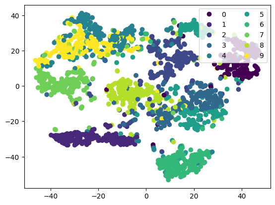
Some good separation, but you can see a few images in the “gaps”. This could be an artifact of dimension reduction, or suggest that we have poor coverage for some covariates.

# Way to calculate data-agnostic radius (probably don't want to do this)
k = 20
n = 2000
d = 10
rho = (1 / math.sqrt(math.pi)) * ((4 * 20 * math.gamma(d / 2 + 1)) / (n)) ** (1 / d)

# Way to calculate data-adaptive radius (most extreme 1% are uncovered)
percent = 0.01
cutoff = int(n * percent)

# Use data adaptive cutoff
cvrg = coverage(mod_preds, radius_type="adaptive")

# Plot the least covered 0.5%
f, axs = plt.subplots(4, 4)
axs = axs.flatten()
for count, i in enumerate(axs):
    i.imshow(np.squeeze(pred[cvrg.indices[count]]), cmap="gray")

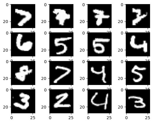
The Coverage tool identified that in this set of 2000 images, there is potential under-coverage when it comes to wonky/ crossed 7s.
Other digits have some undercovered instances, but could be they are just outliers.
More investigation into outlier status is needed, see How to identify outliers and/or anomalies in a dataset for more info.