Assessing the Data Space#
What you’ll do#
You will use DataEval’s coverage function and Clusterer class to identify coverage gaps and outliers in the 2011 VOC dataset.
What you’ll learn#
You’ll learn how to use DataEval’s
coveragefunction andClustererclass to assess a dataset’s data space for coverage gaps and outliers.You’ll learn about the kinds of questions to ask to help you determine if a data point should be removed or additional data collected.
What you’ll need#
Environment Requirements
dataeval[torch]torchvision
Introduction#
Understanding how the data lies within its feature space is a crucial step in evaluating the structure and completeness of your dataset. Before building predictive models, it’s essential to assess how well the data is represented, identify any outliers, and ensure that data groups accurately reflect the underlying distribution.
DataEval has two dedicated methods for identifying and understand the grouping of data, the Clusterer class and the coverage function.
By grouping data points into clusters, you can explore the natural structure of the dataset, revealing hidden patterns and potential anomalies.
The coverage function goes a step further by quantifying how well the clusters represent the entire dataset, ensuring that no significant portion of the feature space is being overlooked.
These techniques are critical for evaluating the quality and representativeness of your data, helping to avoid biases, missing information, or overfitting issues in your models. By focusing on understanding the space your data occupies and how it groups, you can build more robust and reliable models that generalize well in real-world applications.
You’ll begin by installing the necessary libraries to walk through this guide.
# You will need matplotlib for visualing our dataset and numpy to be able to handle the data.
import matplotlib.pyplot as plt
import numpy as np

# You are importing torch in order to create image embeddings.
# You are only using torchvision to load in the dataset.
# If you already have the data stored on your computer in a numpy friendly manner,
# then feel free to load it directly into numpy arrays.
import torch
import torch.nn as nn
import torchvision.transforms.v2 as v2
from torchvision import datasets, models

# Load the classes from DataEval that are helpful for EDA
from dataeval.detectors.linters import Clusterer
from dataeval.metrics.bias import coverage

# Set the random value
rng = np.random.default_rng(213)
Step 1: Load the Data#
You are going to work with the PASCAL VOC 2011 dataset. This dataset is a small curated dataset that was used for a computer vision competition. The images were used for classification, object detection, and segmentation. This dataset was chosen because it has multiple classes and images with a variety of sizes and objects.
If this data is already on your computer you can change the file location from "./data" to wherever the data is stored.
Just remember to also change the download value from True to False.
For the sake of ensuring that this tutorial runs quickly on most computers, you are going to analyze only the training set of the data, which is a little under 6000 images.
# Download the data and then load it as a torch Tensor.
to_tensor = v2.ToImage()
ds = datasets.VOCDetection("./data", year="2011", image_set="train", download=True, transform=to_tensor)
Using downloaded and verified file: ./data/VOCtrainval_25-May-2011.tar
Extracting ./data/VOCtrainval_25-May-2011.tar to ./data
# Verify the size of the loaded dataset
len(ds)
5717
Before moving on, verify that the above code cell printed out 5717 for the size of the dataset.
This ensures that everything is working as needed for the tutorial.
Step 2: Extract Image Embeddings#
Both the Clusterer class and the coverage function expect 2D arrays or in other words a set of 1D images. To flatten our set of 3D images, you will use a neural network to translate the images into 1D embeddings. This will allow you to flatten the dimensions of the image as well as shrink the size of the 1D array, as the images themselves are too large for the Clusterer to handle efficiently. The Clusterer works best when the feature dimension is around 250 or less.
For this guide, you will use a pretrained ResNet18 model and adjust the last layer to be our desired dimension of 128. Also, pretrained torchvision models come with all the necessary information for preprocessing your images correctly for that model.
# Define the embedding network
class EmbeddingNet(nn.Module):
    """
    Simple CNN that repurposes a pretrained ResNet18 model by overwriting the last linear layer.
    Results in a last layer dimension of 128.
    """

    def __init__(self):
        super().__init__()
        self.model = models.resnet18(weights=models.ResNet18_Weights.DEFAULT)
        self.model.fc = nn.Linear(self.model.fc.in_features, 128)

    def forward(self, x):
        x = self.model(x)
        return x


# Initialize the network
embedding_net = EmbeddingNet()
device = torch.device("cuda" if torch.cuda.is_available() else "cpu")
embedding_net.to(device)


# Extract embeddings
def extract_embeddings(dataset, model):
    """Helper function to stack image embeddings from a model"""
    model.eval()

    embeddings = torch.empty(size=(0, 128)).to(device)
    with torch.no_grad():
        images = []
        for i, (img, _) in enumerate(dataset):
            images.append(img)
            if (i + 1) % 64 == 0:
                inputs = torch.stack(images, dim=0).to(device)
                outputs = model(inputs)
                embeddings = torch.vstack((embeddings, outputs))
                images = []
        inputs = torch.stack(images, dim=0).to(device)
        outputs = model(inputs)
        embeddings = torch.vstack((embeddings, outputs))
    return embeddings.detach().cpu().numpy()
Now that the model is defined and initialized, you will reload the dataset with the desired preprocessing for the chosen resnet model. Then you will run the images through the model to get the image embeddings.
# Define pretrained model transformations
preprocess = models.ResNet18_Weights.DEFAULT.transforms()

# Load the dataset
dataset = datasets.VOCDetection("./data", year="2011", image_set="train", download=False, transform=preprocess)

# Create image embeddings
embeddings = extract_embeddings(dataset, embedding_net)
In order for the coverage function to work properly, the embeddings have to be on the unit interval (between 0 and 1). Below normalizes the embeddings to ensure they are on the unit interval.
# Normalize image embeddings
norm_embeddings = (embeddings - embeddings.min()) / (embeddings.max() - embeddings.min())
Step 3: Cluster the Embeddings#
With the images translated into image embeddings and normalized to be on the unit interval,
you can now run the Clusterer to create clusters and identify outliers.
The Clusterer output has 4 keys:
outliers,
potential_outliers,
duplicates,
and near_duplicates.
Outliers are the images which did not fit into a cluster. Potential outliers are images which are on the edge of the cluster, but were not far enough away from the cluster to be considered an outlier. These are good images to compare with the outliers in order to get a sense of what was grouped versus what was not.
In addition to finding outliers and potential outlierts, the Clusterer class can identify duplicates or near duplicates in the dataset. Duplicates are groups of images which are exactly the same. While near duplicates are images which are not exactly the same but very similar, such as the same scene from a slightly different viewpoint or a slightly cropped version of the same image.
# This cell takes about 5-10 minutes to run depending on your hardware

# Initialize the Clusterer class (with the embedded images)
cluster = Clusterer(norm_embeddings)

# Find the outlier images
results = cluster.evaluate()

# View the number of outliers
print(f"Number of outliers: {len(results.outliers)}")
print(f"Number of potential outliers: {len(results.potential_outliers)}")
/builds/jatic/aria/dataeval/.tox/docs/lib/python3.11/site-packages/numpy/core/fromnumeric.py:3504: RuntimeWarning: Mean of empty slice.
  return _methods._mean(a, axis=axis, dtype=dtype,
/builds/jatic/aria/dataeval/.tox/docs/lib/python3.11/site-packages/numpy/core/_methods.py:129: RuntimeWarning: invalid value encountered in scalar divide
  ret = ret.dtype.type(ret / rcount)
Number of outliers: 486
Number of potential outliers: 3508
To get an idea of what the Clusterer class considered an outlier, plot the first 16 images along with their labels.
# Plot random images from each category
fig, axs = plt.subplots(4, 4, figsize=(12, 12))

for i, ax in enumerate(axs.flat):
    # Selected image
    selected_index = results.outliers[i]

    # Grabbing the object names
    names = []
    objects = ds[selected_index][1]["annotation"]["object"]
    for each in objects:
        names.append(each["name"])

    # Plot the corresponding image - need to permute to get channels last for matplotlib
    ax.imshow(np.moveaxis(ds[selected_index][0].numpy(), 0, -1))
    ax.set_title("-".join(set(names)))
    ax.axis("off")

plt.tight_layout()
plt.show()
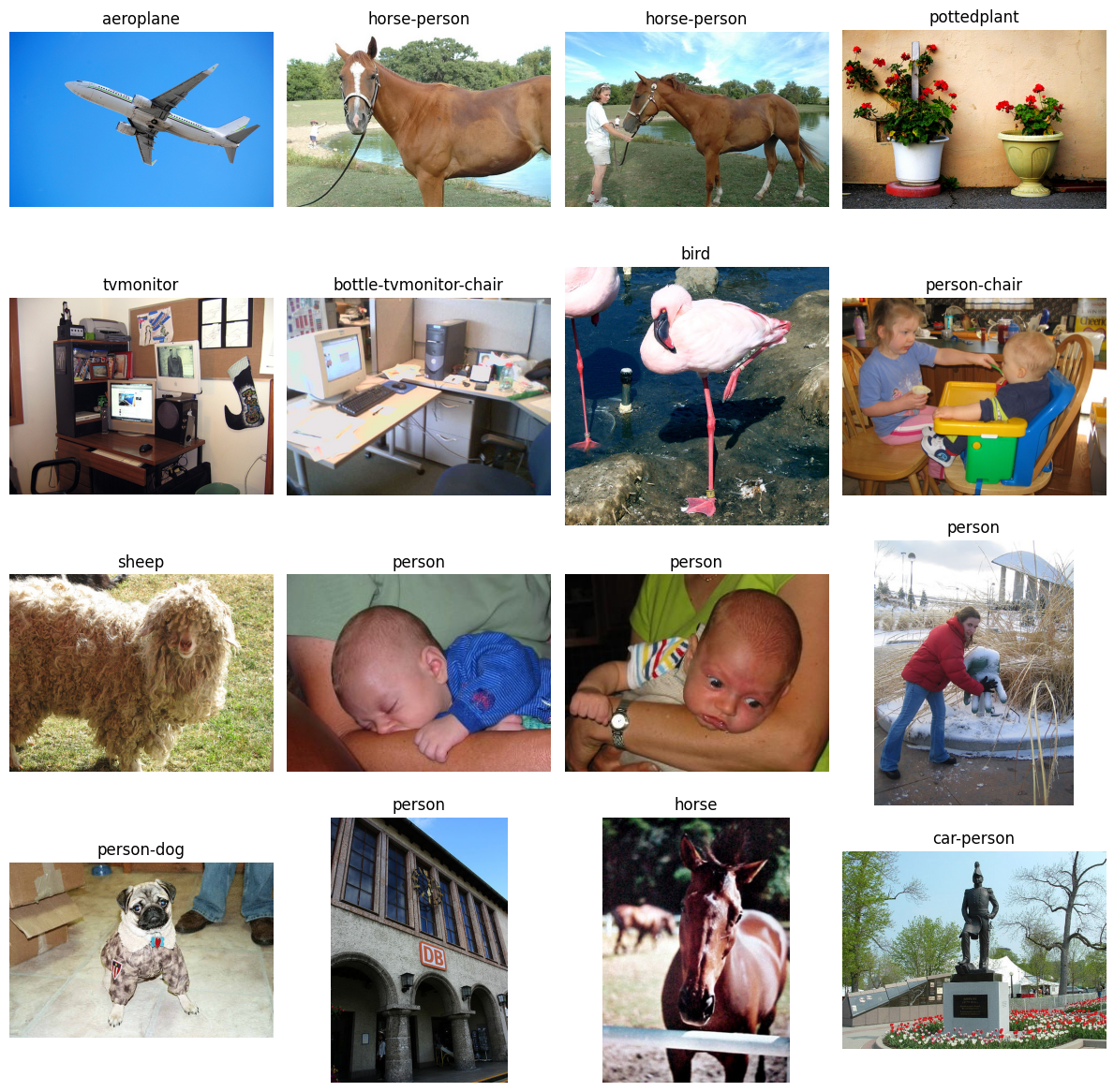
When looking at these images, you want to think about the following questions:
Does this image represent something that would be expected in operation?
Is there commonality to the objects in the images? Such as all the objects are found on the leftside of the images.
Is there commonality to the backgrounds of the images? Such as similar colors, darkness/brightness, places, things (like water or snow).
Is there commonality to the class of objects in the images? Such as a specific pose for person or specific pot color for pottedplant.
You want to address these outliers from the Clusterer with the questions above in mind to determine if they represent actual outliers or just underrepresented samples.
In specific context to the Clusterer, you want to focus on these in a class by class manner,
so thinking about the person class images only in context of the person class, not the dataset as a whole.
A few of the images from above have been analyzed in the context of their classes to help you get an idea of how to process the results.
The first two horse images have a horse with water in the background.
There are 238 total horse images and only 5 of them have water in the background.
So while these images would be operationally relevant if you were trying to detect horses, they are underrepresented in the dataset.
The same goes for the third horse image.
It is one of 4 images that are a close up picture of a horse standing against a fence or railing.
It is most likely flagged as an outlier because it is underrepresented in the dataset.
Likewise with the potted plant, there are only about 4 images with a potted plant up against a solid background out of the 289 potted plant images.
Likely this is also just an underrepresented image.
With the dog image, there are 13 dog images wearing an outfit out of 636 dog images and this is the only one in which the dog is sitting while wearing something, likely an underrepresented image.
With the last two people images that you see, the person is mostly occluded in the last one and they are really small and off to the side in the second to last one.
With the second to last person image, you have to determine how operationally relevant it is.
Are you trying to detect people far away or are you focusing on closer images?
Also, what is the scale at which an object is too small for detection?
With the last one, it is likely that the image could be dropped unless you will often have occlusion when detecting people.
Step 4: Measure the dataset coverage#
From the discussion of the results of the Clusterer class, it was noted that many of the outliers could be underrepresented images in the dataset.
To address this concern, you will use the coverage function to evaluate how well the dataset covers the feature space.
The coverage function identifies data points that are in undercovered regions.
The coverage function output has 3 keys:
indices,
radii, and
critical_value.
Indices contains an array with all of the data points it considers to be uncovered, listing first the most uncovered data point. Radii is an array that contains the defined radius for each data point. Critical value is the calculated threshold value above which the values in radii are considered uncovered.
# Measure the coverage of the embeddings
embedding_coverage = coverage(norm_embeddings)

print(f"Number of uncovered data points: {len(embedding_coverage.indices)}\n{embedding_coverage}")
Number of uncovered data points: 57
CoverageOutput(indices=array([4075, 3005, 3104, 4296, 2495, 1220, 4245, 1365, 2813, 1069,  331,
        292, 3728, 3486,  491, 2412, 4890, 4373, 2557, 1657,  991, 2313,
       3607, 1403, 3602, 3041, 3028, 2829, 1646, 3838, 2065, 3100, 2545,
       2687, 1705, 5659, 3046, 3733, 2550, 3739, 5513, 1723, 4295, 2898,
        909, 1989, 2896, 3892, 5077, 4027, 2527, 1914, 3102, 4699, 2373,
       1709,  417]), radii=array([0.76780375, 0.84465195, 0.84315888, ..., 0.68653826, 0.64807726,
       0.71319266]), critical_value=0.9378492224430178)
According to the coverage function, there are 57 images which are uncovered. You’ll plot the first 16 images along with their labels to see what kind of images are considered uncovered.
# Plot random images from each category
fig, axs = plt.subplots(4, 4, figsize=(12, 12))

for i, ax in enumerate(axs.flat):
    # Selected image
    selected_index = embedding_coverage.indices[i]

    # Grabbing the object names
    names = []
    objects = ds[selected_index][1]["annotation"]["object"]
    for each in objects:
        names.append(each["name"])

    # Plot the corresponding image - need to permute to get channels last for matplotlib
    ax.imshow(np.moveaxis(ds[selected_index][0].numpy(), 0, -1))
    ax.set_title("-".join(set(names)))
    ax.axis("off")

plt.tight_layout()
plt.show()
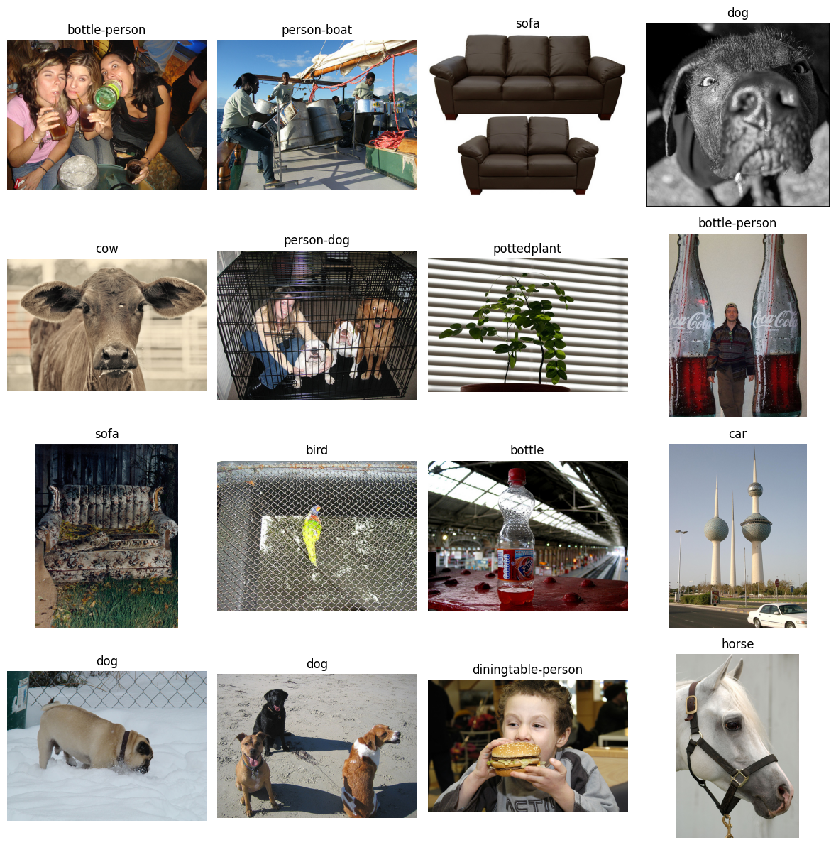
With coverage, you want to ask yourself the same questions that you did with the outliers above:
Does this image represent something that would be expected in operation?
Is there commonality to the objects in the images? Such as all the objects are found on the leftside of the images.
Is there commonality to the backgrounds of the images? Such as similar colors, darkness/brightness, places, things (like water or snow).
Is there commonality to the class of objects in the images? Such as a specific pose for person or specific pot color for pottedplant.
Again, answers to these questions will help you determine if the image is an outlier or an underrepresented region of the dataset. Determining whether an image is an outlier or underrepresented, depends on the task that the data is being used for. The better defined the task, the easier it is to determine whether an image should be thrown out or if additional images of a similar nature need to be collected.
Now that both the Clusterer and the coverage function have been run on this dataset, you’ll compare the results.
uncovered_outliers = [x for x in embedding_coverage.indices if x in results.outliers]
print(
    f"Number of images identified by both functions: {len(uncovered_outliers)} \
        out of {len(embedding_coverage.indices)} possible"
)
print(uncovered_outliers)
Number of images identified by both functions: 54         out of 57 possible
[4075, 3005, 3104, 4296, 2495, 1220, 4245, 1365, 2813, 1069, 331, 292, 3728, 3486, 491, 2412, 4890, 4373, 2557, 1657, 991, 2313, 3607, 1403, 3602, 3041, 3028, 2829, 1646, 3838, 2065, 3100, 2545, 2687, 1705, 5659, 3046, 3733, 2550, 3739, 5513, 1723, 4295, 2898, 909, 1989, 3892, 5077, 4027, 2527, 3102, 2373, 1709, 417]
54 of the 57 uncovered images were also identified by the Clusterer, meaning that they must be analyzed to ensure that they are not outliers first. You can claim the remaining 3 images as uncovered because they were not identified by the Clusterer. Below, you’ll plot the 3 images just to get a look at them.
uncovered_only = [x for x in embedding_coverage.indices if x not in uncovered_outliers]

# Plot random images from each category
fig, axs = plt.subplots(1, 3, figsize=(12, 4))

for i, ax in enumerate(axs.flat):
    # Selected image
    selected_index = uncovered_outliers[i]

    # Grabbing the object names
    names = []
    objects = ds[selected_index][1]["annotation"]["object"]
    for each in objects:
        names.append(each["name"])

    # Plot the corresponding image - need to permute to get channels last for matplotlib
    ax.imshow(np.moveaxis(ds[selected_index][0].numpy(), 0, -1))
    ax.set_title("-".join(set(names)))
    ax.axis("off")

plt.tight_layout()
plt.show()
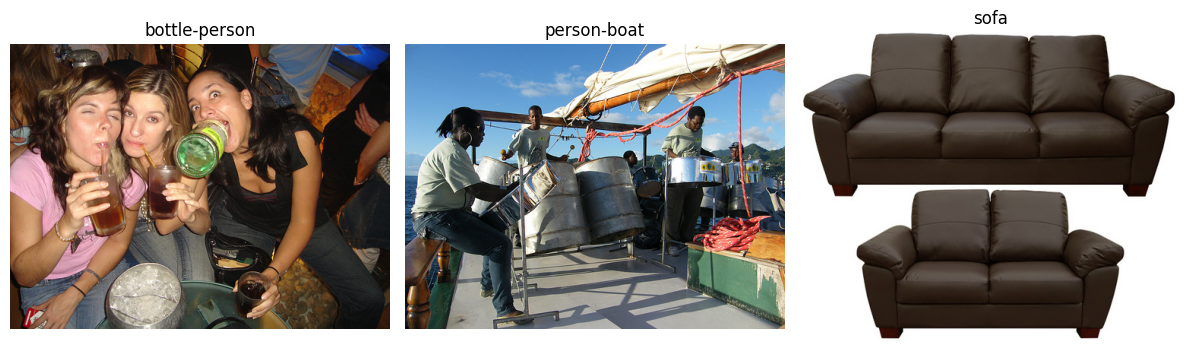
Whether the other 54 images are uncovered or outliers, depend on the task at hand and the answers to the questions above.
Conclusion#
Now comes the fun part, determining what data points are supposed to be in the data set, what points need to be removed, and whether or not you need to collect more data points for a given class or style of image.
The images identified by the Clusterer and coverage stand out from the other images in some way.
DataEval isn’t able to tell you exactly why they stand out, but it highlights the images that you need to check.
You will want to compare each image with other images in that same class to determine whether it is an under-represented image or an image that contains some error and needs to be removed.
As you can see, the DataEval methods are here to help you gain a deep understanding of your dataset and all of it’s strengths and limitations. It is designed to help you create representative and reliable datasets.
Good luck with your data!
What’s Next#
In addition to exploring a dataset in it’s feature space, DataEval offers additional tutorials to help you learn about:
cleaning a dataset with the Data Cleaning Guide,
identifying bias or other factors in a dataset that may influence model performance with the Identifying Bias and Correlations Guide,
and monitoring data for shifts during operation with the Data Monitoring Guide.
To learn more about specific functions or classes, see the Cocept pages.
On your own#
Once you are familiar with DataEval and data analysis, you will want to run this analysis on your own dataset. When you do, make sure that you analyze all of your data and not just the training set.