How to measure dataset sufficiency for image classification
This guide provides a beginner friendly how-to guide to anayze an image classification model’s hypothetical performance.
Estimated time to complete: 10 minutes
Relevant ML stages: Model Development
Relevant personas: ML Engineer
What you’ll do
Evaluate an image classification model’s performance with the MNIST dataset
Define a custom evaluation function with metrics of interest
Project the model’s performance over increasing sample sizes
What you’ll learn
Learn to evaluate a model’s limits for different metrics with the MNIST dataset
Learn to determine how many samples are required to reach specific performance thresholds
Problem Statement
For machine learning tasks, often we would like to evaluate the performance of a model on a small, preliminary dataset. In situations where data collection is expensive, we would like to extrapolate hypothetical performance out to a larger dataset.
DataEval has introduced a method projecting performance via sufficiency curves.
When to use
The Sufficiency class should be used when you would like to extrapolate hypothetical performance. For example, if you have a small dataset, and would like to know if it is worthwhile to collect more data.
What you will need
A particular model architecture.
Metric(s) that we would like to evaluate.
A dataset of interest.
A Python environment with the following packages installed:
tabulate
Setting up
Let’s import the required libraries needed to set up a minimal working example
import os
import random
from collections.abc import Sequence
from typing import cast

import numpy as np
import torch
import torch.nn as nn
import torch.nn.functional as F
import torch.optim as optim
import torchmetrics
from maite_datasets.image_classification import MNIST
from tabulate import tabulate
from torch.utils.data import DataLoader, Dataset, Subset

from dataeval.data import Select
from dataeval.data.selections import Limit
from dataeval.workflows import Sufficiency

np.random.seed(0)
np.set_printoptions(formatter={"float": lambda x: f"{x:0.4f}"})
torch.manual_seed(0)
torch.set_float32_matmul_precision("high")
device = "cuda" if torch.cuda.is_available() else "cpu"
torch._dynamo.config.suppress_errors = True

random.seed(0)
torch.use_deterministic_algorithms(True)
os.environ["CUBLAS_WORKSPACE_CONFIG"] = ":4096:8"
Load data and define functions
Load the MNIST data and create the training and test datasets. For the purposes of this example, we will use subsets of the training (2500) and test (500) data.
# Configure the dataset transforms

transforms = [
    lambda x: x / 255.0,  # scale to [0, 1]
    lambda x: x.astype(np.float32),  # convert to float32
]

# Download the mnist dataset and apply the transforms and subset the data

train_ds = Select(MNIST(root="./data", image_set="train", transforms=transforms,download=True),selections=[Limit(2500)])  # fmt: skip # noqa: E501
test_ds = Select(MNIST(root="./data", image_set="test", transforms=transforms, download=True), selections=[Limit(500)])
Next, we define the network architecture we will be using.
# Define our network architecture
class Net(nn.Module):
    def __init__(self):
        super().__init__()
        self.conv1 = nn.Conv2d(1, 6, 5)
        self.conv2 = nn.Conv2d(6, 16, 5)
        self.fc1 = nn.Linear(6400, 120)
        self.fc2 = nn.Linear(120, 84)
        self.fc3 = nn.Linear(84, 10)

    def forward(self, x):
        x = F.relu(self.conv1(x))
        x = F.relu(self.conv2(x))
        x = torch.flatten(x, 1)  # flatten all dimensions except batch
        x = F.relu(self.fc1(x))
        x = F.relu(self.fc2(x))
        x = self.fc3(x)
        return x


# Compile the model
model = torch.compile(Net().to(device))

# Type cast the model back to Net as torch.compile returns a Unknown
# Nothing internally changes from the cast; we are simply signaling the type
model = cast(Net, model)
Finally, we define our custom training and evaluation functions. Sufficiency requires that the evaluation function returns a dictionary of the results.
def custom_train(model: nn.Module, dataset: Dataset, indices: Sequence[int]):
    # Defined only for this testing scenario
    criterion = torch.nn.CrossEntropyLoss().to(device)
    optimizer = optim.SGD(model.parameters(), lr=0.01, momentum=0.9)
    epochs = 10

    # Define the dataloader for training
    dataloader = DataLoader(Subset(dataset, indices), batch_size=8)

    for epoch in range(epochs):
        for batch in dataloader:
            # Load data/images to device
            X = torch.Tensor(batch[0]).to(device)
            # Load one-hot encoded targets/labels to device
            y = torch.argmax(torch.asarray(batch[1], dtype=torch.int).to(device), dim=1)
            # Zero out gradients
            optimizer.zero_grad()
            # Forward propagation
            outputs = model(X)
            # Compute loss
            loss = criterion(outputs, y)
            # Back prop
            loss.backward()
            # Update weights/parameters
            optimizer.step()
def custom_eval(model: nn.Module, dataset: Dataset) -> dict[str, float]:
    # Metrics of interest
    metrics = {
        "Accuracy": torchmetrics.Accuracy(task="multiclass", num_classes=10).to(device),
        "AUROC": torchmetrics.AUROC(task="multiclass", num_classes=10).to(device),
        "TPR at 0.5 Fixed FPR": torchmetrics.ROC(task="multiclass", average="macro", num_classes=10).to(device),
    }
    result = {}
    # Set model layers into evaluation mode
    model.eval()
    dataloader = DataLoader(dataset, batch_size=8)
    # Tell PyTorch to not track gradients, greatly speeds up processing
    with torch.no_grad():
        for batch in dataloader:
            # Load data/images to device
            X = torch.Tensor(batch[0]).to(device)
            # Load one-hot encoded targets/labels to device
            y = torch.argmax(torch.asarray(batch[1], dtype=torch.int).to(device), dim=1)
            preds = model(X)
            for metric in metrics.values():
                metric.update(preds, y)
        # Compute ROC curve
        false_positive_rate, true_positive_rate, _ = metrics["TPR at 0.5 Fixed FPR"].compute()
        # determine interval to examine
        desired_rate = 0.5
        closest_desired_index = torch.argmin(torch.abs(false_positive_rate - desired_rate)).item()
        # return corresponding tpr value
        result["TPR at 0.5 Fixed FPR"] = true_positive_rate[closest_desired_index].cpu()
        result["Accuracy"] = metrics["Accuracy"].compute().cpu()
        result["AUROC"] = metrics["AUROC"].compute().cpu()
    return result
Initialize sufficiency metric
Attach the custom training and evaluation functions to the Sufficiency metric and define the number of models to train in parallel (stability), as well as the number of steps along the learning curve to evaluate.
# Instantiate sufficiency metric
suff = Sufficiency(
    model=model,  # type: ignore
    train_ds=train_ds,  # type: ignore
    test_ds=test_ds,  # type: ignore
    train_fn=custom_train,
    eval_fn=custom_eval,
    runs=5,
    substeps=10,
)
Evaluate Sufficiency
Now we can evaluate the metric to train the models and produce the learning curve.
# Train & test model
output = suff.evaluate()
W0808 22:58:13.622000 2481 torch/_inductor/utils.py:1250] [0/0] Not enough SMs to use max_autotune_gemm mode
# Print out sufficiency output in a table format
formatted = {"Steps": output.steps, **output.averaged_measures}
print(tabulate(formatted, headers=list(formatted), tablefmt="pretty"))
+-------+----------------------+---------------------+--------------------+
| Steps | TPR at 0.5 Fixed FPR |      Accuracy       |       AUROC        |
+-------+----------------------+---------------------+--------------------+
|  25   |  0.785096275806427   | 0.22600000202655793 | 0.7452809929847717 |
|  41   |  0.9053672790527344  | 0.5151999950408935  | 0.8521784663200378 |
|  69   |  0.9683709859848022  | 0.6319999933242798  | 0.9186212301254273 |
|  116  |  0.9749770641326905  | 0.7096000075340271  | 0.9391248464584351 |
|  193  |  0.9881328701972961  | 0.7600000023841857  | 0.9602133989334106 |
|  322  |  0.9956899046897888  | 0.8212000012397767  | 0.9746083378791809 |
|  538  |  0.9975358009338379  | 0.8763999938964844  | 0.9881841897964477 |
|  898  |  0.9987630724906922  | 0.9036000013351441  | 0.9914544463157654 |
| 1498  |  0.9983268022537232  |  0.919599997997284  | 0.9931858301162719 |
| 2500  |  0.999147379398346   | 0.9335999965667725  | 0.9946498990058898 |
+-------+----------------------+---------------------+--------------------+
# Print out projected output values
projection = output.project([1000, 2500, 5000])
projected = {"Steps": projection.steps, **projection.averaged_measures}
print(tabulate(projected, list(projected), tablefmt="pretty"))
+-------+----------------------+--------------------+--------------------+
| Steps | TPR at 0.5 Fixed FPR |      Accuracy      |       AUROC        |
+-------+----------------------+--------------------+--------------------+
| 1000  |  0.9973940156715576  | 0.8993037608365085 | 0.9897572002570741 |
| 2500  |  0.9976878325718003  | 0.9210708577875996 | 0.9927793577301677 |
| 5000  |  0.9977410755183604  | 0.9300243572841603 | 0.9937331475927237 |
+-------+----------------------+--------------------+--------------------+
# Plot the output using the convenience function
_ = output.plot()
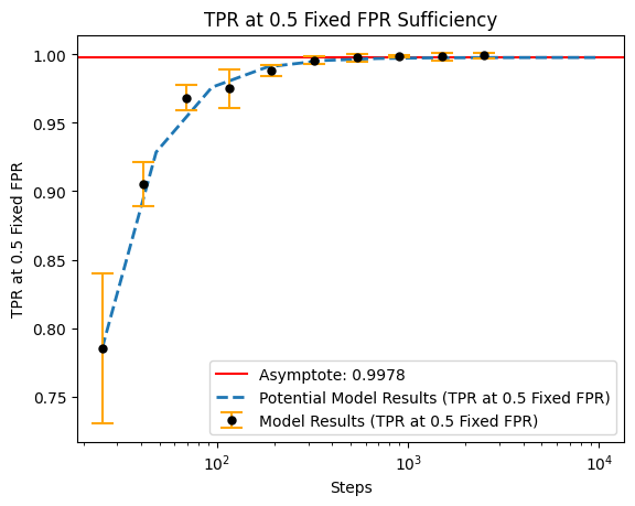
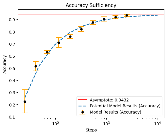
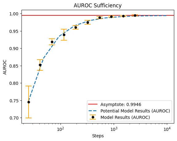
Results
Using these learning curves, we can project performance under much larger datasets (with the same models).
Predicting sample requirements
We can also predict the amount of training samples required to achieve specific performance thresholds.
Let’s say we wanted to see how many samples are needed to hit 90%, 93%, and 99% accuracy, area under the receiver operating characteristic, and true positive rate at a fixed false positive rate of 0.5.
# Initialize the array of desired thresholds to apply to all metrics
desired_values = np.array([0.90, 0.93, 0.99])
metrics = ["Accuracy", "AUROC", "TPR at 0.5 Fixed FPR"]
evaluated_metrics = {}

for metric in metrics:
    evaluated_metrics[metric] = desired_values
# Evaluate the learning curve to infer the needed amount of training data
samples_needed = output.inv_project(evaluated_metrics)
/dataeval/src/dataeval/outputs/_workflows.py:151: UserWarning: Number of samples could not be determined for target(s): [0.99] with asymptote of 0.9432286805829774
  warnings.warn(
# Print the amount of needed data needed to achieve the thresholds
for metric, samples in samples_needed.items():
    print(f"{metric}")
    for index, sample_size in enumerate(samples):
        print(
            f"To achieve {int(evaluated_metrics[metric][index] * 100)}% {metric},"
            f" {int(sample_size)} samples are needed."
        )
    print()
Accuracy
To achieve 90% Accuracy, 1021 samples are needed.
To achieve 93% Accuracy, 4987 samples are needed.
To achieve 99% Accuracy, -1 samples are needed.

AUROC
To achieve 90% AUROC, 61 samples are needed.
To achieve 93% AUROC, 87 samples are needed.
To achieve 99% AUROC, 1049 samples are needed.

TPR at 0.5 Fixed FPR
To achieve 90% TPR at 0.5 Fixed FPR, 39 samples are needed.
To achieve 93% TPR at 0.5 Fixed FPR, 48 samples are needed.
To achieve 99% TPR at 0.5 Fixed FPR, 170 samples are needed.
The projection shows that given the current model, hitting an accuracy of 99% is improbable.