Image Statistical Analysis¶

The image statistics functions assist with understanding the dataset. These can be used to get a big picture view of the dataset and it’s underlying distribution. These functions create the data distribution that the Outliers class uses to identify outliers.

What are the statistical analysis functions¶

There are seven different DataEval stat functions for analyzing a dataset:

• boxratiostats

• dimensionstats

• hashstats

• imagestats

• labelstats

• pixelstats

• visualstats

The information below includes what each function does and the statistical analysis metrics that are included in each function.

boxratiostats¶

The boxratiostats() function calculates the ratio of the bounding box outputs to the image outputs. This function can be used with the output from:

• dimensionstats()

• pixelstats()

• visualstats()

This function requires both a bounding box output and an image output from the above mentioned stat functions.

This function can be used in conjunction with the Outliers class to determine if there are issues with any of the images in the dataset.

imagestats¶

The imagestats() function provides an easy way to run the pixelstats and visualstats on the images of a dataset or over each channel of the images of a dataset.

dimensionstats¶

The dimensionstats() function is an aggregate metric that calculates various dimension based statistics for each individual image:

This function expects the image in a CxHxW format and uses this standard format to populate the width, height and channels metrics.

This function can be used in conjunction with the Outliers class to determine if there are any issues with any of the images in the dataset.

hashstats¶

The hashstats() function is an aggregate metric that calculates various hash values for each individual image:

This function can be used in conjunction with the Duplicates class in order to identify duplicate images.

labelstats¶

The labelstats() function provides summary statistics across classes and labels:

pixelstats¶

The pixelstats() function is an aggregate metric that calculates normal statistics about pixel values for each individual image:

This function can be used in conjunction with the Outliers class to determine if there are any issues with any of the images in the dataset.

visualstats¶

The visualstats() function is an aggregate metric that calculates visual quality statistics for each individual image:

This function can be used in conjunction with the Outliers class to determine if there are any issues with any of the images in the dataset.

When to use the statistical analysis functions¶

The functions are automatically called when using Outliers.evaluate on data. Therefore, the functions themselves don’t usually need to be called on the data. However, there are a few scenarios that lend themselves to using the functions independently:

• When multiple sets of data as well as the combined set are to be analyzed, it can be easier to run the stat functions on each individual set of data and then pass in the outputs to the Outlier class in each of the desired data combinations for analysis.

• When comparing the resulting data distribution between two or more datasets to determine how similar the datasets are.

• When visualizing the resulting data distribution after using one or more of the stat functions.

Example visualizing the resulting data distribution¶

The output for each function contains a plot function which plots a histogram of the data results, except for the hashstats function whose results are grouped lists and has no visualization function, and the labelstats function whose results can be visualized instead with the to_table function.

Example code and result for the imagestats function for images:

# Load the statistic metric from DataEval
from dataeval.metrics.stats import imagestats

# Loading in the PASCAL VOC 2011 dataset for this example
to_tensor = v2.ToImage()
ds = VOCDetection(
    "./data",
    year="2011",
    image_set="train",
    download=True,
    transform=to_tensor,
)

# This stat function takes about 1-3 minutes to run depending on your hardware

# Calculate the imagestats for the images
# Note: the stat function expects the images as a dataset
#       with images in the (C,H,W) format
stats = imagestats(ds)

# Visualize the results
stats.plot(log=True)

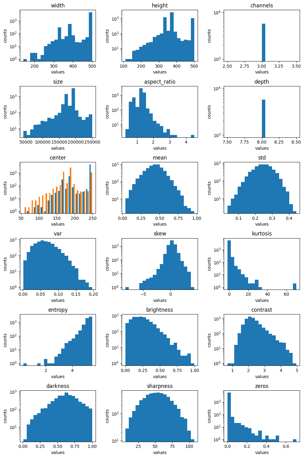
Example code and result for the imagestats function for channels per image:

# Load the statistic metric from DataEval
from dataeval.metrics.stats import imagestats

# Loading in the PASCAL VOC 2011 dataset for this example
to_tensor = v2.ToImage()
ds = VOCDetection(
    "./data",
    year="2011",
    image_set="train",
    download=True,
    transform=to_tensor,
)

# This stat function takes about 1-3 minutes to run depending on your hardware

# Calculate the imagestats per channel for the images
# Note: the stat function expects the images as a dataset
#       with images in the (C,H,W) format
ch_stats = imagestats(ds, per_channel=True)

# Visualize the results
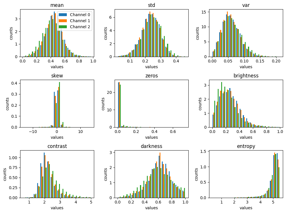
ch_stats.plot(log=False, channel_limit=3)

Using the visualization for a quick analysis¶

Visualizing the distribution of values for each metric allows one to quickly inspect the metrics for unusual distributions. In general, each metric should follow either a normal distribution or a uniform distribution.

With a uniform distribution, you want to notice if any of the plots have areas that are a lot shorter or a lot taller than the rest of the values.

With a normal distribution, you are looking at the edges of the bell curve to see if the values near the edges of the plot raise up or if there are gaps between the edge values and the next value in.

When analyzing the visualizations by channel, you should not be interested in the overall shape of these plots but in the comparison of the shape across each of the individual channels. You want to see if the same shape holds across each channel or if there are large differences between the channels. This is important because discrepancies across channels can help detect image processing errors and channel bias.

For example, below is a quick analysis of the above example plots.

In regards to the imagestats plot, there are a few key insights:

1. The channel metric has only one value, 3, which is interesting since some of the images in the dataset are greyscale, and greyscale images usually only have 1 channel.

2. The entropy, zeros, kurtosis, and contrast metrics are single-tailed and all of them have a long tail which indicates that the images whose values are in the edges of the tail are potentially problematic.

3. Size, aspect ratio, variance, skew, brightness and darkness have skewed or off-center distributions which is another sign of problematic images.

4. Mean, standard deviation and sharpness appear to have a normal distribution and none have an extended tail, which is a good sign.

While these insights don’t identify the exact images that may be problematic, they highlight where to focus on with further analysis.

In regards to the per-channel plot, the only insight is that there is very little difference across the channels for each metric. Therefore, there are no additional concerns beyond those from the imagestats plot.