Out of distribution data¶

What is out-of-distribution (OOD)?¶

Out-of-Distribution (OOD) refers to data samples that deviate significantly from the statistical patterns of the reference dataset used to train a model.

In unsupervised anomaly detection, the model learns the “normal” patterns from a reference training set (In-Distribution). When it encounters operational data that does not conform to these learned patterns, it flags them as outliers.

OOD data typically falls into two categories:

• Structural Anomalies: The input is corrupted, broken, or contains localized defects (e.g., a scratch on a product surface, sensor noise, or digital artifacts).

• Semantic Shift: The input represents a valid object or state that simply belongs to a class not seen during training (e.g., a “walking” motion in a dataset consisting only of “running”).

When to use OOD detection¶

OOD detection methods should be used when you need to identify individual samples in a dataset that are qualitatively different from those in a reference (training) dataset. Typical use cases include:

• Operational Monitoring: Determining if new operational data contains samples significantly different from training data

• Data Quality Control: Identifying corrupted, damaged, or anomalous samples in production pipelines

• Novel Class Detection: Finding operationally relevant classes or sub-classes not present in training data

• Model Reliability: Preventing model degradation when novel samples represent a significant portion of operational data

This type of detection is critical because models are likely to degrade rapidly if OOD data represents a significant portion of operational inputs.

Two fundamental approaches¶

DataEval provides two conceptual frameworks for OOD detection, each with distinct strengths and computational characteristics:

Reconstruction-based detection¶

Core Principle: Learn to recreate the data.

Reconstruction-based methods work by learning a compressed representation of the normal data distribution and attempting to reconstruct input samples. The fundamental assumption is that the model will successfully reconstruct in-distribution samples but fail to accurately reconstruct OOD samples that lie outside the learned manifold.

How it works:

1. The model learns to compress high-dimensional input data into a lower-dimensional latent representation

2. It then attempts to reconstruct the original input from this compressed form

3. The reconstruction error (difference between input and output) serves as the OOD score

4. High reconstruction error indicates the sample is likely OOD

Key characteristics:

• Requires training a neural network model on reference data

• Learns the underlying structure and patterns of the data distribution

• Can capture complex, non-linear relationships in the data

• Provides both instance-level and feature-level anomaly scores

• Training time ranges from moderate to high depending on model complexity

DataEval Implementation: OODReconstruction

Distance-based detection (K-nearest neighbors)¶

Core Principle: Measure proximity to known examples.

Distance-based methods operate directly on pre-computed feature embeddings, using the principle that OOD samples will be far from normal samples in embedding space. Rather than learning to reconstruct data, these methods memorize the reference distribution and compare new samples against it.

How it works:

1. Reference embeddings from normal data are stored or indexed

2. For each new sample, the method computes distances to its nearest neighbors in the reference set

3. Samples far from their nearest neighbors are considered OOD

4. The average distance to k-nearest neighbors serves as the OOD score

Key characteristics:

• Requires pre-computed embeddings (from a separate feature extractor)

• No neural network training required - non-parametric approach

• Fast to “fit” (just indexes the reference embeddings)

• Fast inference using efficient nearest neighbor search

• Assumes embeddings capture meaningful semantic similarity

• Provides only instance-level scores

DataEval Implementation: OODKNeighbors

Reconstruction-based methods in detail¶

Different reconstruction architectures are suited for different types of OOD data. DataEval’s OODReconstruction class supports multiple architectures that can be automatically detected or explicitly specified.

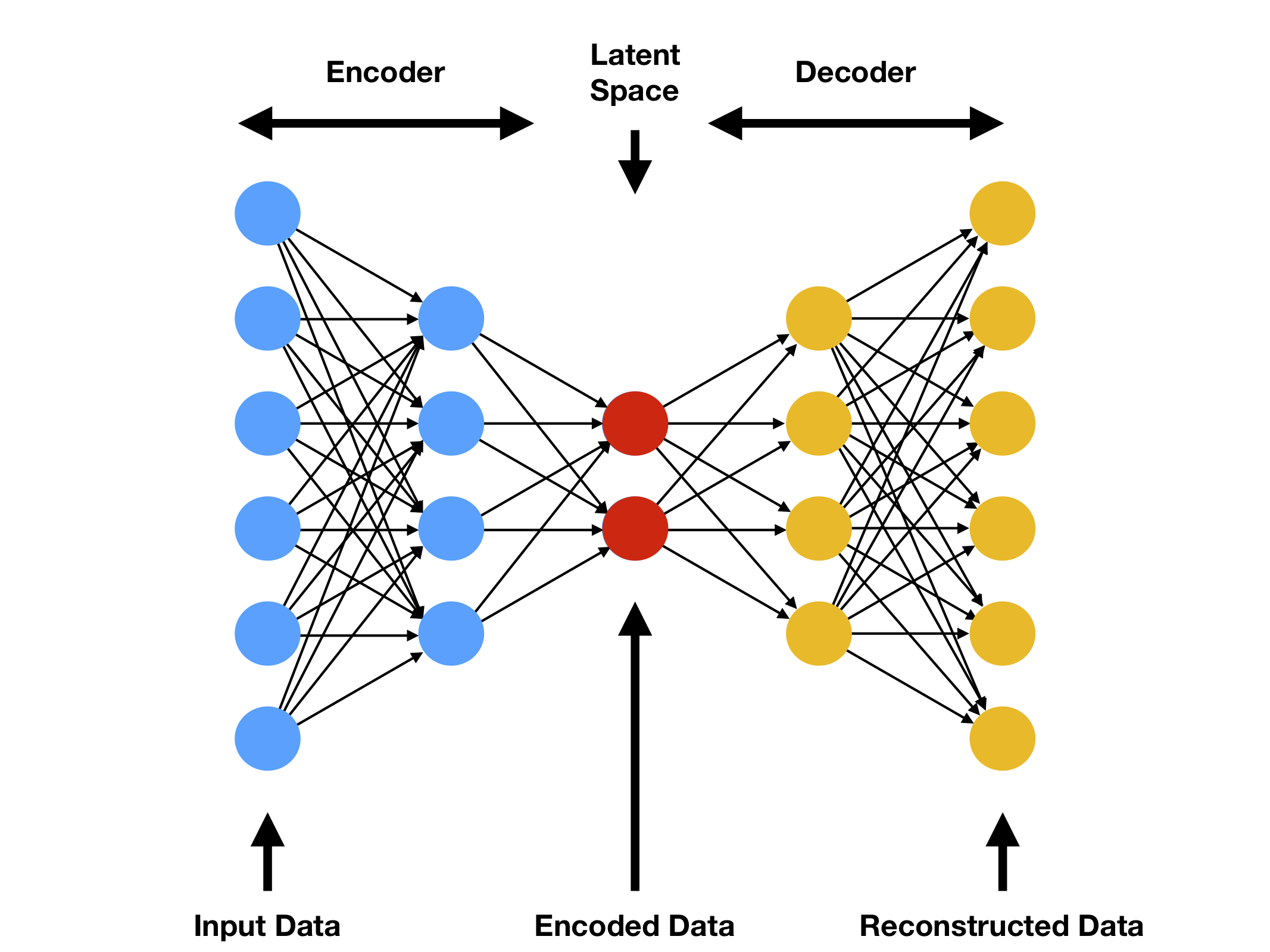
Autoencoder (AE)¶

Mechanism: Reconstruction Error.

An Autoencoder compresses high-dimensional input data into a lower-dimensional latent vector and attempts to reconstruct it back to the original input.

(https://www.compthree.com/blog/autoencoder/)

• Theory: The model learns the specific “manifold” (structure) of the training data. If it encounters an OOD sample, it fails to compress and reconstruct it accurately because it lacks the learned features to describe that specific anomaly.

• Metric: Mean Squared Error (MSE) between the input and the reconstruction.

• Latent Space: Deterministic encoding - each input maps to a single point in latent space.

• Best For: Structural defects like cracks, noise, corruptions, or broken parts.

Variational autoencoder (VAE)¶

Mechanism: Probabilistic Likelihood (ELBO).

A VAE adds a probabilistic constraint to the latent space, forcing the latent vectors to follow a continuous distribution (usually a Standard Normal distribution).

• Theory: While standard AEs only care about reconstruction accuracy, VAEs also care about how “likely” a data point is to occur under the model’s learned probability distribution. It regularizes the latent space to be smooth and continuous.

• Metric: Evidence Lower Bound (ELBO). A low ELBO score indicates the sample is statistically improbable.

• Latent Space: Probabilistic encoding - each input is encoded as a distribution (mean and variance), introducing controlled randomness.

• Best For: Probabilistic shifts, noisy biological data, or subtle statistical shifts.

AE/VAE with GMM (deep mixture models)¶

Mechanism: Density Estimation & Energy.

These models combine the dimensionality reduction of an autoencoder with the clustering capability of a Gaussian Mixture Model (GMM).

• Theory: Real-world data is often multimodal (e.g., distinct clusters for “Day Mode” vs. “Night Mode”). A standard AE or VAE attempts to compress these into a single distribution center. By adding a GMM, the model explicitly learns multiple distinct “centers” of density in the latent space.

• Metric: A combined score of Reconstruction Error (structure) + GMM Energy (density). The GMM energy measures how well a sample fits into one of the learned Gaussian components. Scores are combined using sensor fusion (z-score normalization and weighted combination).

• Latent Space: Explicitly modeled as a mixture of Gaussians, where each component represents a distinct mode in the data.

• Best For: Multimodal data with distinct sub-populations (e.g., different machine operating speeds, day/night imagery).

Configuration: The OODReconstructionConfig class allows tuning of score fusion parameters:

• gmm_weight: Weight for GMM component (default 0.5, range [0, 1])

• gmm_score_mode: Fusion method (“standardized” or “percentile”)

Distance-based methods in detail¶

K-nearest neighbors (KNN) in embedding space¶

Mechanism: Proximity to Reference Samples.

The OODKNeighbors detector works by computing how far a test sample is from its nearest neighbors in a reference set of normal embeddings.

Theory: The assumption is that in-distribution samples form dense clusters in embedding space, while OOD samples lie in sparse regions far from these clusters. The method leverages pre-trained feature extractors (e.g., from supervised learning, self-supervised learning, or foundation models) that map inputs to meaningful embeddings.

Distance Metrics:

• Cosine Distance: Measures angular similarity, effective when embeddings are normalized or direction matters more than magnitude.

• Euclidean Distance: Measures absolute distance in embedding space, effective when magnitude represents meaningful differences.

How to use:

from dataeval.shift import OODKNeighbors
from dataeval import Embeddings

# Create embeddings using a pre-trained model
train_emb = Embeddings(train_data, model=your_model)
test_emb = Embeddings(test_data, model=your_model)

# Fit detector and predict
detector = OODKNeighbors(k=10, distance_metric="cosine")
detector.fit(train_emb, threshold_perc=95.0)
result = detector.predict(test_emb)

Advantages:

• Training-free: No neural network optimization required

• Fast inference: Modern KNN libraries use efficient indexing

• Interpretable: Scores directly correspond to distance in embedding space

• Flexible: Works with any embedding source (ResNet, CLIP, DINO, etc.)

Considerations:

• Embedding quality: Performance heavily depends on the quality of the pre-trained embeddings

• Dimensionality: High-dimensional embeddings may suffer from curse of dimensionality

• Memory: Requires storing or indexing all reference embeddings

• Choice of k: Too small may be sensitive to noise, too large may miss local structure

Comparison of approaches¶

High-level comparison: Reconstruction vs. distance¶

Reconstruction methods comparison¶

Choosing the right approach¶

When to use reconstruction-based methods¶

Use OODReconstruction when:

• You have sufficient training data representing normal behavior

• You need to understand where anomalies occur (feature-level detection)

• You want to learn task-specific representations

• You don’t have access to pre-trained embeddings

• Your data has complex structural patterns that need to be learned

Example use cases:

• Manufacturing quality control (detecting defects in product images)

• Medical imaging (identifying abnormal tissue structures)

• Sensor data analysis (detecting equipment malfunctions)

When to use distance-based methods¶

Use OODKNeighbors when:

• You have high-quality pre-trained embeddings available

• You want fast deployment without model training

• You need very fast inference times

• Your reference dataset is too small to train a reconstruction model

• You’re working with domains where foundation models provide strong embeddings (e.g., natural images with CLIP/DINO)

Example use cases:

• Content moderation (flagging unusual images using CLIP embeddings)

• Ecological monitoring (detecting rare species in wildlife camera traps)

• Zero-shot OOD detection (leveraging pre-trained vision models)

Hybrid approach¶

In practice, both approaches can be complementary:

1. Two-stage detection: Use distance-based methods for fast initial screening, then apply reconstruction-based methods for detailed analysis of flagged samples

2. Ensemble methods: Combine scores from both approaches for more robust detection

3. Feature extraction + reconstruction: Use a pre-trained encoder as the embedding source, then train only a lightweight decoder for reconstruction-based scoring

Tutorials and further reading¶

For hands-on examples and detailed comparisons:

• Identify Out-of-Distribution Samples Tutorial - Comprehensive comparison of all methods on MNIST digits

For related concepts:

• Drift Detection

• Machine Learning Lifecycle

References¶

[1] Van Looveren, A., Klaise, J., Vacanti, G., Cobb, O., Scillitoe, A., Samoilescu, R., & Athorne, A. (2024). Alibi Detect: Algorithms for outlier, adversarial and drift detection (0.12.1.dev0)

[2] Kuan, J., & Mueller, J. (2022). Back to the Basics: Revisiting Out-of-Distribution Detection Baselines. arXiv preprint arXiv:2207.03061.