How to run clustering analysis¶

Problem Statement¶

Data does not typically come labeled and labeling/verifying labels is a time and resource intensive process. Exploratory data analysis (EDA) can often be enhanced by splitting data into similar groups.

Clustering is a method which groups data in the format of (samples, features). This can be used with images or image embeddings as long as the arrays are flattened to only contain 2 dimensions.

The cluster function utilizes a clustering algorithm based on the HDBSCAN algorithm. The Outliers and Duplicates detectors can then analyze the cluster results to identify outliers and duplicates.

When to use¶

The clustering workflow can be used during the EDA process to perform the following:

• group a dataset into clusters

• verify labeling as a quality control

• identify outliers in your dataset using the Outliers detector

• identify duplicates in your dataset using the Duplicates detector

What you will need¶

1. A 2 dimensional dataset (samples, features)

2. A Python environment with the following packages installed:

   • dataeval

   • matplotlib

This could be a set of flattened images or image embeddings. We recommend using image embeddings (with the feature dimension being <=1000).

Getting Started¶

Let’s import the required libraries needed to set up a minimal working example.

import matplotlib.pyplot as plt
import numpy as np
import sklearn.datasets as dsets

from dataeval.core import cluster
from dataeval.quality import Duplicates, Outliers

Loading in data¶

For the purposes of this demonstration, we are just going to create a generic set of blobs for clustering.

This is to help show all of the clustering functionality in one how-to.

# Creating 5 clusters
test_data, labels = dsets.make_blobs(
    n_samples=100,
    centers=[(-1.5, 1.8), (-1, 3), (0.8, 2.1), (2.8, 1.5), (2.5, 3.5)],
    cluster_std=0.3,
    random_state=33,
)  # type: ignore

Because the clustering result can be used to detect duplicate and outlier data, we are going to modify the dataset to contain a few duplicate datapoints and an outlier.

test_data[71] = [1, 5]
test_data[79] = test_data[24]
test_data[63] = test_data[58] + 1e-5
labels[79] = labels[24]
labels[63] = labels[58]

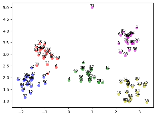
Visualizing the clusters¶

# Mapping from labels to colors
label_to_color = np.array(["b", "r", "g", "y", "m", "gray"])

# Translate labels to colors using vectorized operation
color_array = label_to_color[labels]

# Set plotting parameters
plot_kwds = {"alpha": 0.5, "s": 50, "linewidths": 0}

# Create scatter plot
plt.scatter(test_data.T[0], test_data.T[1], c=color_array, **plot_kwds)

# Annotate each point in the scatter plot
for i, (x, y) in enumerate(test_data):
    plt.annotate(str(i), (x, y), textcoords="offset points", xytext=(0, 1), ha="center")

# Verify the number of datapoints and that the shape is 2 dimensional
print("Number of samples: ", len(test_data))
print("Array shape:", test_data.ndim)

Number of samples:  100
Array shape: 2

Cluster the data¶

We are now ready to cluster the data and inspect the results.
There are two different clustering methods, “kmeans” and “hdbscan”. These are selected via the algorithm parameter, with “hdbscan” being the default.

# Evaluate the clusters
clusters = cluster(test_data, algorithm="hdbscan", n_clusters=5)

clusters["clusters"]

array([ 2,  0,  2,  2,  2,  3,  3,  4,  4,  0,  3,  2,  4,  2,  1,  2,  2,
        4,  3,  4,  0,  3,  2,  1,  2,  1,  3,  4,  0,  4,  2,  1,  4,  4,
        1,  3,  2,  3,  1,  4,  1,  1,  3,  1,  3,  3,  2,  4,  3,  1,  4,
        4,  4,  3,  1,  4,  0,  2,  0,  1,  3,  3,  1,  0,  4,  3,  2,  2,
        1,  0,  4, -1,  1,  3,  4,  4,  4,  0,  0,  2,  0,  0,  0,  0,  1,
        0,  1,  2,  1,  1,  3,  0,  4,  0,  4,  2,  1,  0,  0,  2])

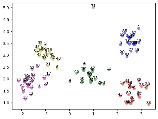
Visualize the resulting clusters¶

# Using the same plotting as above
color_array = label_to_color[clusters["clusters"]]
plt.scatter(test_data.T[0], test_data.T[1], c=color_array, **plot_kwds)

# Annotate each point in the scatter plot
for i, (x, y) in enumerate(test_data):
    plt.annotate(str(i), (x, y), textcoords="offset points", xytext=(0, 1), ha="center")

Results¶

We can list out each category followed by the number of items in the category and then display those items on the line below.

For the outlier results, the clusterer provides a list of all points that it found to be an outlier.

For the duplicates and near duplicate results, the clusterer provides a list of sets of points which it identified as duplicates.

# Show results using the new detector classes
duplicates_detector = Duplicates()
duplicates_result = duplicates_detector.from_clusters(clusters)
print("exact image duplicates: ", duplicates_result.items.exact)
print("near image duplicates: ", duplicates_result.items.near)

outliers_detector = Outliers()
outliers_result = outliers_detector.from_clusters(test_data, clusters, threshold=3)
print("outliers: ", outliers_result.issues)

exact image duplicates:  [[24, 79], [58, 63]]
near image duplicates:  [NearDuplicateGroup([0, 13, 22, 67, 87, 95], methods=['cluster']), NearDuplicateGroup([3, 24], methods=['cluster']), NearDuplicateGroup([8, 27, 29], methods=['cluster']), NearDuplicateGroup([10, 65], methods=['cluster']), NearDuplicateGroup([16, 99], methods=['cluster']), NearDuplicateGroup([17, 21], methods=['cluster']), NearDuplicateGroup([19, 64], methods=['cluster']), NearDuplicateGroup([30, 57], methods=['cluster']), NearDuplicateGroup([31, 86], methods=['cluster']), NearDuplicateGroup([33, 76], methods=['cluster']), NearDuplicateGroup([36, 66], methods=['cluster']), NearDuplicateGroup([39, 55], methods=['cluster']), NearDuplicateGroup([40, 72, 96], methods=['cluster']), NearDuplicateGroup([41, 62], methods=['cluster']), NearDuplicateGroup([58, 83], methods=['cluster']), NearDuplicateGroup([80, 81, 93], methods=['cluster']), NearDuplicateGroup([82, 97], methods=['cluster'])]
outliers:  shape: (1, 3)
┌─────────┬──────────────────┬──────────────┐
│ item_id ┆ metric_name      ┆ metric_value │
│ ---     ┆ ---              ┆ ---          │
│ i64     ┆ cat              ┆ f64          │
╞═════════╪══════════════════╪══════════════╡
│ 71      ┆ cluster_distance ┆ 4.000434     │
└─────────┴──────────────────┴──────────────┘

We can see that there was one outlier and there are also 2 sets of exact duplicates and 17 sets of near duplicates.