How to detect undersampled data subsets¶

Problem Statement¶

For most computer vision tasks like image classification and object detection, we often have a lot of images, but certain subsets of the images can be undersampled, such as label, style within a label, etc. A way to detect this regional sparsity is through coverage analysis.

To help with this, DataEval has introduced a coverage() function, that provides a user with example images which have few similar instances within the provided dataset.

When to use¶

The coverage function should be used when you have lots of images, but only a small fraction from certain regimes/labels.

What you will need¶

Image classification dataset.
Autoencoder trained on image classification dataset for dimension reduction.
A Python environment with the following packages installed:
- dataeval
- tabulate

Setting up¶

Let’s import the required libraries needed to set up a minimal working example

import matplotlib.pyplot as plt
import numpy as np
import torch
import torch.nn as nn
from maite_datasets.image_classification import MNIST
from sklearn.manifold import TSNE

from dataeval import Embeddings, Metadata
from dataeval.core import coverage_adaptive
from dataeval.extractors import TorchExtractor
from dataeval.selection import Limit, Select

print(torch.cuda.is_available())

True

Load the data¶

Load the MNIST data and create the training dataset.

# Set seeds
torch.manual_seed(14)

transforms = [
    lambda x: x / 255.0,  # scale to [0, 1]
    lambda x: (x - 0.1307) / 0.3081,  # normalize
    lambda x: x.astype(np.float32),  # convert to float32
]

# MNIST with mean 0 unit variance
train_ds = MNIST(root="./data", image_set="train", transforms=transforms, download=True)

# Select a subset of the dataset
subset = Select(train_ds, Limit(2000))

In this tutorial, we will use an autoencoder to reduce the dimension of the MNIST images.

# Define model architecture
class Autoencoder(nn.Module):
    def __init__(self):
        super().__init__()
        self.encoder = nn.Sequential(
            # 28 x 28
            nn.Conv2d(1, 4, kernel_size=5),
            # 4 x 24 x 24
            nn.ReLU(True),
            nn.Conv2d(4, 8, kernel_size=5),
            nn.ReLU(True),
            # 8 x 20 x 20 = 3200
            nn.Flatten(),
            nn.Linear(3200, 10),
            # 10
            nn.Sigmoid(),
        )
        self.decoder = nn.Sequential(
            # 10
            nn.Linear(10, 400),
            # 400
            nn.ReLU(True),
            nn.Linear(400, 4000),
            # 4000
            nn.ReLU(True),
            nn.Unflatten(1, (10, 20, 20)),
            # 10 x 20 x 20
            nn.ConvTranspose2d(10, 10, kernel_size=5),
            # 24 x 24
            nn.ConvTranspose2d(10, 1, kernel_size=5),
            # 28 x 28
            nn.Sigmoid(),
        )

    def forward(self, x):
        x = self.encoder(x)
        x = self.decoder(x)
        return x

    def encode(self, x):
        x = self.encoder(x)
        return x

For computational reasons, we will simply load the trained autoencoder.

# The trained autoencoder was trained for 1000 epochs
sd = torch.load("models/ae", weights_only=True)
model = Autoencoder()
model.load_state_dict(sd)

<All keys matched successfully>

For the purposes of this example, we will take only the first 2000 entries of the data.

# Create extractor using the autoencoder's encoder portion
extractor = TorchExtractor(model.encoder)

# Calculate the embeddings and extract the labels from the dataset
embeddings = Embeddings(subset, extractor=extractor, batch_size=64)
labels = Metadata(subset).class_labels

To visualize the encodings, we will use TSNE on them to view separation.

# Visualize 10d as 2d with TSNE
tsne = TSNE(n_components=2)
red_dim = tsne.fit_transform(embeddings)

# Plot results with color being label
fig, ax = plt.subplots()
scatter = ax.scatter(
    x=red_dim[:, 0],
    y=red_dim[:, 1],
    c=labels,
    label=labels,
)
ax.legend(*scatter.legend_elements(), loc="upper right", ncols=2)
plt.show()

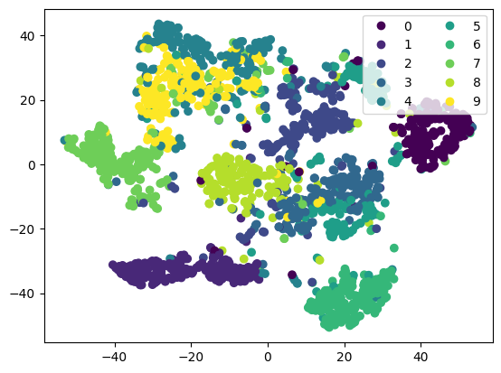
../_images/9a7e92b87230d98f5a9b33816c4b0d1f415fcfa4cc0e2c5603485ebe62733faf.png

Some good separation, but you can see a few images in the “gaps”. This could be an artifact of dimension reduction, or suggest that we have poor coverage for some covariates.

# Use data adaptive cutoff
cvrg = coverage_adaptive(embeddings, 20, 0.01)

# Plot the least covered 1%
f, axs = plt.subplots(4, 5, figsize=(5, 5))
axs = axs.flatten()
for count, i in enumerate(axs):
    idx = cvrg["uncovered_indices"][count]
    i.imshow(np.squeeze(train_ds[idx][0]), cmap="gray")
    i.set_axis_off()
    i.title.set_text(int(labels[idx]))

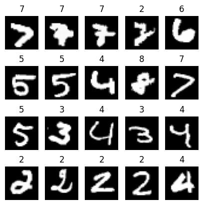
../_images/a47abc6e8f7707dcab3aa39c91c191bee833dfd2329c5fd436707446b779ec7c.png

The Coverage tool identified that in this set of 2000 images, there is potential under-coverage when it comes to wonky 2s and 7s. Other digits have some undercovered instances, but could be they are just outliers.