Identify out-of-distribution samples¶

This guide demonstrates how to identify out-of-distribution (OOD) samples using reconstruction-based methods with different model architectures.

Estimated time to complete: 10-15 minutes

Relevant ML stages: Monitoring, Data Engineering

Relevant personas: Machine Learning Engineer, T&E Engineer, Data Scientist

What you’ll do¶

Train different reconstruction models (AE, VAE) for OOD detection
Use Gaussian Mixture Models (GMM) to enhance OOD detection
Compare KNN-based OOD detection with cosine and Euclidean distance metrics
Compare model performance on different OOD scenarios
Visualize reconstruction quality and OOD scores

What you’ll learn¶

When to use Autoencoder (AE) vs Variational Autoencoder (VAE) for OOD detection
How GMM in latent space improves OOD detection
When to choose cosine vs Euclidean distance for KNN-based detection
How to interpret OOD scores and set appropriate thresholds
Different use cases for each model configuration

What you’ll need¶

Knowledge of Python
Basic understanding of PyTorch and neural networks
Understanding of autoencoders (helpful but not required)

Introduction¶

Out-of-distribution (OOD) detection is critical for ensuring model reliability in production. When models encounter data that differs significantly from their training distribution, predictions become unreliable. This tutorial demonstrates seven different approaches to OOD detection:

Reconstruction-Based Methods:

Standard Autoencoder (AE): Simple reconstruction-based detection using mean squared error
Variational Autoencoder (VAE): Probabilistic approach with regularized latent space
AE with GMM: Enhanced detection by modeling latent space with Gaussian Mixture Models
VAE with GMM: Combining probabilistic encoding with GMM for robust detection

Distance-Based Methods:

KNN with Cosine Distance: Measures angular similarity in learned embeddings
KNN with Euclidean Distance: Measures straight-line distance in learned embeddings

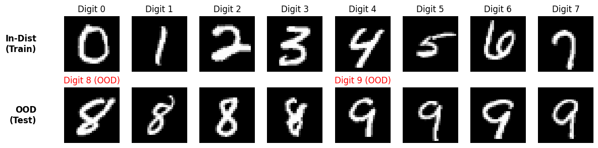
For this tutorial, you’ll use the MNIST dataset of handwritten digits. You’ll train models to recognize digits 0-7 and test their ability to detect digits 8-9 as out-of-distribution samples.

Setup¶

First, install the required packages and import necessary libraries.

Important note on expected results¶

OOD detection performance depends heavily on how different the OOD data is from the in-distribution data:

Easy OOD: Completely different data (e.g., cats vs dogs) → near 100% detection
Hard OOD: Similar data (e.g., digit 8 vs digit 0, both have circles) → lower detection rates

In this tutorial, we use digits 8-9 as OOD against training on 0-7. This is a moderately challenging scenario because:

Digit 8 shares circular shapes with 0, 6
Digit 9 shares curves with 3, 5

Therefore, you should expect:

In-distribution accuracy: ~95% (matching our threshold)
OOD detection rates: Variable (20-80%), depending on model and similarity
Score separation: OOD scores higher than in-dist, but distributions may overlap

This reflects real-world scenarios where OOD data often shares features with training data!

try:
    import google.colab  # noqa: F401

    %pip install -q dataeval torchvision
except Exception:
    pass

from typing import cast

import matplotlib.pyplot as plt
import numpy as np
import torch
from maite_datasets.image_classification import CIFAR10, MNIST

import dataeval
from dataeval import Embeddings
from dataeval.extractors import TorchExtractor
from dataeval.selection import ClassFilter, Limit, Select, Shuffle
from dataeval.shift import OODKNeighbors, OODReconstruction
from dataeval.utils.models import AE, VAE, GMMDensityNet
from dataeval.utils.preprocessing import rescale, resize, to_canonical_grayscale

# Set random seeds for reproducibility
dataeval.config.set_seed(173, all_generators=True)

# Set default batch size
dataeval.config.set_batch_size(64)

# Set default torch device
device = torch.device("cuda" if torch.cuda.is_available() else "cpu")
print(f"Using device: {device}")

Using device: cuda

Prepare the data¶

You’ll load the MNIST dataset and split it into in-distribution (digits 0-7) and out-of-distribution (digits 8-9) samples.

def normalize(x):
    return x.astype(np.float32) / 255.0


in_dist_digits = [0, 1, 2, 3, 4, 5, 6, 7]
out_of_dist_digits = [8, 9]


mnist_train = Select(
    MNIST("./data", image_set="train", download=True, transforms=normalize),
    selections=[Shuffle(), Limit(10000), ClassFilter(in_dist_digits)],
)
mnist_test_in = Select(
    MNIST("./data", image_set="test", download=True, transforms=normalize),
    selections=[Shuffle(), Limit(1000), ClassFilter(in_dist_digits)],
)
mnist_test_ood = Select(
    MNIST("./data", image_set="test", download=True, transforms=normalize),
    selections=[Shuffle(), Limit(1000), ClassFilter(out_of_dist_digits)],
)

print(f"Training set size: {len(mnist_train)}")
print(f"Test set size: {len(mnist_test_in)}")
print(f"Test set size: {len(mnist_test_ood)}")

# Set the input shape (MNIST images are 28x28 grayscale)
input_shape = (1, 28, 28)

Training set size: 10000
Test set size: 1000
Test set size: 1000

# Extract data and labels from prefiltered datasets
def extract_data_labels(dataset):
    """Extract images and labels from a dataset."""
    data, labels = [], []

    for img, label_probs, _ in dataset:
        label = np.argmax(label_probs)
        data.append(img)
        labels.append(label)

    return np.stack(data), np.asarray(labels)


# Extract training and test data (already filtered for correct classes)
train_in, train_in_labels = extract_data_labels(mnist_train)
test_in, test_in_labels = extract_data_labels(mnist_test_in)
test_ood, test_ood_labels = extract_data_labels(mnist_test_ood)

print(f"Training in-distribution: {train_in.shape}")
print(f"Test in-distribution: {test_in.shape}")
print(f"Test out-of-distribution: {test_ood.shape}")

Training in-distribution: (10000, 1, 28, 28)
Test in-distribution: (1000, 1, 28, 28)
Test out-of-distribution: (1000, 1, 28, 28)

# Visualize some in-distribution and OOD samples
fig, axes = plt.subplots(2, 8, figsize=(12, 3))

# Show in-distribution samples (0-7) - one of each digit
for digit in range(8):
    # Find the first occurrence of this digit
    idx = (train_in_labels == digit).nonzero()[0][0]
    axes[0, digit].imshow(train_in[idx].squeeze(), cmap="gray")
    axes[0, digit].axis("off")
    axes[0, digit].set_title(f"Digit {digit}")

# Show OOD samples (8-9) - 4 of each
for i in range(8):
    digit = 8 if i < 4 else 9
    idx = (test_ood_labels == digit).nonzero()[0][(i % 4) * 50]
    axes[1, i].imshow(test_ood[idx].squeeze(), cmap="gray")
    axes[1, i].axis("off")
    if i % 4 == 0:
        axes[1, i].set_title(f"Digit {digit} (OOD)", color="red")

axes_text_kwargs = {"ha": "right", "va": "center", "fontsize": 12, "fontweight": "bold"}
axes[0, 0].text(-0.5, 0.5, "In-Dist\n(Train)", transform=axes[0, 0].transAxes, **axes_text_kwargs)
axes[1, 0].text(-0.5, 0.5, "OOD\n(Test)", transform=axes[1, 0].transAxes, **axes_text_kwargs)

plt.tight_layout()
plt.show()

../_images/d8fe56fe3b5d1d650207bf8ea188218efedcafc2e5eae880ccafbf32eaa7b78e.png

K-nearest neighbors (KNN) for OOD detection¶

KNN-based OOD detection is a simple yet effective approach that utilizes a pretrained model to create learned embeddings. It works by measuring how far test samples are from their nearest neighbors in the training data. Samples that are far from all training samples are likely OOD.

Use Case: Fast baseline for OOD detection without model training, interpretable distance-based scoring.

⚠️ Important Note on Embeddings: KNN performance depends entirely on the quality of the embeddings you provide:

Better embeddings = better OOD detection: Use task-specific, well-trained models
For images: ResNets, Vision Transformers (ViT), CLIP, or custom CNNs trained on similar data
For text: BERT, sentence transformers, domain-specific language models
For time series: LSTMs, Transformers trained on temporal data
For tabular: MLPs or autoencoders trained on your feature space

This tutorial trains a simple CNN for demonstration, but using pretrained models (e.g., ImageNet-pretrained ResNet) would likely improve results significantly.

# Define a simple CNN for learning embeddings
class EmbeddingNet(torch.nn.Module):
    """Simple CNN that learns embeddings for digit classification."""

    def __init__(self, embedding_dim=64):
        super().__init__()
        self.embedding_dim = embedding_dim

        # Convolutional layers
        self.conv_layers = torch.nn.Sequential(
            torch.nn.Conv2d(1, 32, kernel_size=3, padding=1),
            torch.nn.ReLU(),
            torch.nn.MaxPool2d(2),  # 28x28 -> 14x14
            torch.nn.Conv2d(32, 64, kernel_size=3, padding=1),
            torch.nn.ReLU(),
            torch.nn.MaxPool2d(2),  # 14x14 -> 7x7
        )

        # Embedding layer
        self.embedding = torch.nn.Sequential(
            torch.nn.Flatten(),
            torch.nn.Linear(64 * 7 * 7, 128),
            torch.nn.ReLU(),
            torch.nn.Linear(128, embedding_dim),
        )

        # Classification head (for training only)
        self.classifier = torch.nn.Linear(embedding_dim, 8)  # 8 digit classes (0-7)

    def forward(self, x, return_embedding=False):
        """Forward pass. Returns embeddings if return_embedding=True, else logits."""
        emb = self.embedding(self.conv_layers(x))
        return emb if return_embedding else self.classifier(emb)

# Create and train the embedding model
embedding_model = EmbeddingNet(embedding_dim=64).to(device)
optimizer = torch.optim.Adam(embedding_model.parameters(), lr=0.001)
criterion = torch.nn.CrossEntropyLoss()

print("Training embedding model for digit classification...")
print(f"Embedding dimension: {embedding_model.embedding_dim}")

# Train for a few epochs
num_epochs = 3
batch_size = 256

for epoch in range(num_epochs):
    embedding_model.train()
    total_loss, correct, total = 0, 0, 0

    # Create batches
    num_batches = len(train_in) // batch_size
    for i in range(num_batches):
        start_idx = i * batch_size
        end_idx = start_idx + batch_size

        batch_imgs = torch.as_tensor(train_in[start_idx:end_idx], device=device)
        batch_labels = torch.as_tensor(train_in_labels[start_idx:end_idx], device=device)

        # Forward pass
        optimizer.zero_grad()
        logits = embedding_model(batch_imgs)
        loss = criterion(logits, batch_labels)

        # Backward pass
        loss.backward()
        optimizer.step()

        total_loss += loss.item()
        _, predicted = torch.max(logits.data, 1)
        total += batch_labels.size(0)
        correct += (predicted == batch_labels).sum().item()

    avg_loss = total_loss / num_batches
    accuracy = 100 * correct / total
    print(f"Epoch {epoch + 1}/{num_epochs} - Loss: {avg_loss:.4f}, Accuracy: {accuracy:.2f}%")

print("✓ Embedding model trained!")

Training embedding model for digit classification...
Embedding dimension: 64

Epoch 1/3 - Loss: 0.9002, Accuracy: 72.40%

Epoch 2/3 - Loss: 0.2188, Accuracy: 93.23%

Epoch 3/3 - Loss: 0.1353, Accuracy: 95.87%
✓ Embedding model trained!

# Create extractor using the trained embedding model
knn_extractor = TorchExtractor(embedding_model, device=device)

# Get embeddings for all datasets
print("Extracting embeddings...")
train_in_emb = Embeddings(train_in, extractor=knn_extractor)
test_in_emb = Embeddings(test_in, extractor=knn_extractor)
test_ood_emb = Embeddings(test_ood, extractor=knn_extractor)

print(f"Training embeddings shape: {train_in_emb.shape}")
print(f"Test in-dist embeddings shape: {test_in_emb.shape}")
print(f"Test OOD embeddings shape: {test_ood_emb.shape}")

Extracting embeddings...
Training embeddings shape: (10000, 8)
Test in-dist embeddings shape: (1000, 8)
Test OOD embeddings shape: (1000, 8)

# Create KNN detector with learned embeddings
ood_knn_cos = OODKNeighbors(k=10, distance_metric="cosine")

print("\nFitting KNN detector with learned embeddings...")
ood_knn_cos.fit(train_in_emb, threshold_perc=95.0)
print("Done!")

Fitting KNN detector with learned embeddings...

Done!

# Get predictions with learned embeddings
knn_cos_result_in = ood_knn_cos.predict(test_in_emb)
knn_cos_result_ood = ood_knn_cos.predict(test_ood_emb)

# Calculate detection accuracy
in_acc_knn = 100 * (1 - knn_cos_result_in.is_ood.mean())
ood_rate_knn = 100 * knn_cos_result_ood.is_ood.mean()

print("\n--- KNN Cosine (Embeddings) Results ---")
print(f"In-distribution correctly identified: {in_acc_knn:.1f}%")
print(f"OOD samples detected: {ood_rate_knn:.1f}%")
print(f"Average score (in-dist): {knn_cos_result_in.instance_score.mean():.4f}")
print(f"Average score (OOD): {knn_cos_result_ood.instance_score.mean():.4f}")

--- KNN Cosine (Embeddings) Results ---
In-distribution correctly identified: 95.2%
OOD samples detected: 36.8%
Average score (in-dist): 0.0150
Average score (OOD): 0.0472

KNN with Euclidean distance¶

Euclidean distance measures the straight-line distance between points in the embedding space. Unlike cosine similarity, which only considers the angle between vectors, Euclidean distance also accounts for their magnitude. This makes it better suited for embeddings where the scale of the vectors carries meaningful information.

# Create KNN detector with Euclidean distance
ood_knn_euc = OODKNeighbors(k=10, distance_metric="euclidean")

print("Fitting KNN (Euclidean) detector with learned embeddings...")
ood_knn_euc.fit(train_in_emb, threshold_perc=95.0)
print("Done!")

Fitting KNN (Euclidean) detector with learned embeddings...

Done!

# Get predictions with Euclidean distance
knn_euc_result_in = ood_knn_euc.predict(test_in_emb)
knn_euc_result_ood = ood_knn_euc.predict(test_ood_emb)

# Calculate detection accuracy
in_acc_knn_euc = 100 * (1 - knn_euc_result_in.is_ood.mean())
ood_rate_knn_euc = 100 * knn_euc_result_ood.is_ood.mean()

print("\n--- KNN Euclidean (Embeddings) Results ---")
print(f"In-distribution correctly identified: {in_acc_knn_euc:.1f}%")
print(f"OOD samples detected: {ood_rate_knn_euc:.1f}%")
print(f"Average score (in-dist): {knn_euc_result_in.instance_score.mean():.4f}")
print(f"Average score (OOD): {knn_euc_result_ood.instance_score.mean():.4f}")

--- KNN Euclidean (Embeddings) Results ---
In-distribution correctly identified: 96.0%
OOD samples detected: 21.3%
Average score (in-dist): 2.4977
Average score (OOD): 3.6957

Standard autoencoder (AE) for OOD detection¶

The simplest approach uses a standard autoencoder that learns to reconstruct normal (in-distribution) images. When presented with OOD data, reconstruction error increases, signaling anomalous samples.

Use Case: Fast, simple OOD detection when you have well-separated distributions and don’t need probabilistic interpretations.

⚠️ Important Note on Model Architecture: This tutorial uses a simple, generic AE architecture provided by DataEval for demonstration purposes. In production:

Design architectures for your data type: CNNs for images, LSTMs/Transformers for sequences, MLPs for tabular data
Match complexity to your problem: Deeper networks for complex data, simpler for basic patterns
Tune hyperparameters: Latent dimension size, layer widths, activation functions, etc.
Your model choice significantly impacts OOD detection performance

The DataEval OODReconstruction class works with any PyTorch model you provide—customize it for best results.

# Create and configure the autoencoder
ae_model = AE(input_shape=input_shape)

# Configure training parameters
config = OODReconstruction.Config(
    epochs=3,
    batch_size=64,
    threshold_perc=95.0,  # 95% of training data considered normal
)

# Initialize OOD detector
ood_ae = OODReconstruction(ae_model, device=device, config=config)

print("Training Standard Autoencoder...")
print(f"Model type detected: {ood_ae.model_type}")
print(f"Using GMM: {ood_ae.use_gmm}")

Training Standard Autoencoder...
Model type detected: ae
Using GMM: False

# Train the model on in-distribution data
ood_ae.fit(train_in)

# Get predictions
ae_result_in = ood_ae.predict(test_in)
ae_result_ood = ood_ae.predict(test_ood)

# Calculate detection accuracy
in_acc_ae = 100 * (1 - ae_result_in.is_ood.mean())
ood_rate_ae = 100 * ae_result_ood.is_ood.mean()

print("\n--- Standard AE Results ---")
print(f"In-distribution correctly identified: {in_acc_ae:.1f}%")
print(f"OOD samples detected: {ood_rate_ae:.1f}%")
print(f"Average score (in-dist): {ae_result_in.instance_score.mean():.4f}")
print(f"Average score (OOD): {ae_result_ood.instance_score.mean():.4f}")

# Validation: Check if OOD scores are higher than in-dist scores
score_separation = ae_result_ood.instance_score.mean() - ae_result_in.instance_score.mean()
print(f"\nScore separation (OOD - In-Dist): {score_separation:.4f}")
if score_separation > 0:
    print("✓ Expected: OOD samples have higher scores than in-distribution samples")
else:
    print("⚠ Warning: OOD scores should be higher than in-distribution scores")

# Check if we're near the target threshold
if 90 <= in_acc_ae <= 98:
    print(f"✓ Expected: ~95% of in-distribution samples correctly identified (got {in_acc_ae:.1f}%)")
else:
    print(f"⚠ Note: Expected ~95% in-dist accuracy, got {in_acc_ae:.1f}%")

--- Standard AE Results ---
In-distribution correctly identified: 93.2%
OOD samples detected: 26.9%
Average score (in-dist): 0.0039
Average score (OOD): 0.0059

Score separation (OOD - In-Dist): 0.0020
✓ Expected: OOD samples have higher scores than in-distribution samples
✓ Expected: ~95% of in-distribution samples correctly identified (got 93.2%)

Variational autoencoder (VAE) for OOD detection¶

VAEs learn a probabilistic latent representation, which provides better generalization and more structured latent spaces compared to standard AEs. This can improve OOD detection, especially when in-distribution data has high variability.

Use Case: When you need a more robust latent representation or when your in-distribution data has significant variance.

# Create and configure the VAE
vae_model = VAE(input_shape=input_shape)

# Initialize OOD detector (auto-detects as VAE)
ood_vae = OODReconstruction(vae_model, device=device, config=config)

print("Training Variational Autoencoder...")
print(f"Model type detected: {ood_vae.model_type}")
print(f"Using GMM: {ood_vae.use_gmm}")

Training Variational Autoencoder...
Model type detected: vae
Using GMM: False

# Train the VAE
ood_vae.fit(train_in)

# Evaluate VAE performance
vae_result_in = ood_vae.predict(test_in)
vae_result_ood = ood_vae.predict(test_ood)

in_acc_vae = 100 * (1 - vae_result_in.is_ood.mean())
ood_rate_vae = 100 * vae_result_ood.is_ood.mean()

print("\n--- VAE Results ---")
print(f"In-distribution correctly identified: {in_acc_vae:.1f}%")
print(f"OOD samples detected: {ood_rate_vae:.1f}%")
print(f"Average score (in-dist): {vae_result_in.instance_score.mean():.4f}")
print(f"Average score (OOD): {vae_result_ood.instance_score.mean():.4f}")

--- VAE Results ---
In-distribution correctly identified: 93.9%
OOD samples detected: 4.8%
Average score (in-dist): 0.1365
Average score (OOD): 0.1419

Autoencoder with GMM for enhanced OOD detection¶

Adding a Gaussian Mixture Model (GMM) to the latent space provides an additional signal for OOD detection. The GMM models the density of the latent representations, and samples with low density are likely to be OOD. This combines reconstruction error with density estimation using sensor fusion: both components are standardized (z-score normalized) and combined with configurable weighting.

Use Case: When you need higher detection accuracy and have complex in-distribution data that naturally clusters into multiple groups.

⚠️ Important: GMM fusion parameters (gmm_weight and gmm_score_mode) significantly impact performance. The default gmm_weight=0.7 favors the GMM component, which typically works well. Experiment with values in [0.5, 0.9] for your data.

# Create AE with GMM density network
# The latent dimension is auto-computed by AE
ae_model_gmm = AE(input_shape=input_shape)
latent_dim = cast(int, ae_model_gmm.encoder.flatten[1].out_features)

# Create GMM density network with 3 components
gmm_density_net = GMMDensityNet(latent_dim=latent_dim, n_gmm=3)
ae_model_gmm.gmm_density_net = gmm_density_net

# Configure training parameters
config_gmm = OODReconstruction.Config(
    epochs=3,
    batch_size=64,
    threshold_perc=95.0,  # 95% of training data considered normal
    gmm_weight=0.7,  # For GMM models: balance reconstruction (30%) and GMM energy (70%)
    gmm_score_mode="standardized",  # Use z-score normalization for score fusion
)

# Initialize OOD detector (auto-detects GMM usage)
ood_ae_gmm = OODReconstruction(ae_model_gmm, device=device, config=config_gmm)

print("Training Autoencoder with GMM...")
print(f"Model type detected: {ood_ae_gmm.model_type}")
print(f"Using GMM: {ood_ae_gmm.use_gmm}")
print(f"Latent dimension: {latent_dim}")
print(f"Number of GMM components: {gmm_density_net.n_gmm}")

Training Autoencoder with GMM...
Model type detected: ae
Using GMM: True
Latent dimension: 256
Number of GMM components: 3

# Train the AE+GMM model
ood_ae_gmm.fit(train_in)

# Evaluate AE+GMM performance
ae_gmm_result_in = ood_ae_gmm.predict(test_in)
ae_gmm_result_ood = ood_ae_gmm.predict(test_ood)

in_acc_ae_gmm = 100 * (1 - ae_gmm_result_in.is_ood.mean())
ood_rate_ae_gmm = 100 * ae_gmm_result_ood.is_ood.mean()

print("\n--- AE + GMM Results ---")
print(f"In-distribution correctly identified: {in_acc_ae_gmm:.1f}%")
print(f"OOD samples detected: {ood_rate_ae_gmm:.1f}%")
print(f"Average score (in-dist): {ae_gmm_result_in.instance_score.mean():.4f}")
print(f"Average score (OOD): {ae_gmm_result_ood.instance_score.mean():.4f}")

--- AE + GMM Results ---
In-distribution correctly identified: 94.3%
OOD samples detected: 16.7%
Average score (in-dist): 0.0059
Average score (OOD): 0.6881

VAE with GMM for maximum robustness¶

Combining VAE’s probabilistic latent space with GMM density estimation provides the most sophisticated OOD detection approach. This is particularly effective when you need high reliability and have sufficient computational resources.

Use Case: Production systems where false negatives (missing OOD samples) are costly, and you need maximum detection reliability.

# Create VAE with GMM density network
vae_model_gmm = VAE(input_shape=input_shape)
vae_latent_dim = vae_model_gmm.latent_dim

# Create GMM density network
gmm_density_net_vae = GMMDensityNet(latent_dim=vae_latent_dim, n_gmm=3)
vae_model_gmm.gmm_density_net = gmm_density_net_vae

# Initialize OOD detector
ood_vae_gmm = OODReconstruction(vae_model_gmm, device=device, config=config_gmm)

print("Training VAE with GMM...")
print(f"Model type detected: {ood_vae_gmm.model_type}")
print(f"Using GMM: {ood_vae_gmm.use_gmm}")
print(f"Latent dimension: {vae_latent_dim}")
print(f"Number of GMM components: {gmm_density_net_vae.n_gmm}")

Training VAE with GMM...
Model type detected: vae
Using GMM: True
Latent dimension: 256
Number of GMM components: 3

# Train the VAE+GMM model
ood_vae_gmm.fit(train_in)

# Evaluate VAE+GMM performance
vae_gmm_result_in = ood_vae_gmm.predict(test_in)
vae_gmm_result_ood = ood_vae_gmm.predict(test_ood)

in_acc_vae_gmm = 100 * (1 - vae_gmm_result_in.is_ood.mean())
ood_rate_vae_gmm = 100 * vae_gmm_result_ood.is_ood.mean()

print("\n--- VAE + GMM Results ---")
print(f"In-distribution correctly identified: {in_acc_vae_gmm:.1f}%")
print(f"OOD samples detected: {ood_rate_vae_gmm:.1f}%")
print(f"Average score (in-dist): {vae_gmm_result_in.instance_score.mean():.4f}")
print(f"Average score (OOD): {vae_gmm_result_ood.instance_score.mean():.4f}")

--- VAE + GMM Results ---
In-distribution correctly identified: 94.0%
OOD samples detected: 16.4%
Average score (in-dist): 0.0001
Average score (OOD): 0.6730

Compare all methods¶

Now let’s visualize and compare the performance of all six approaches.

# Summary comparison
methods = ["KNN\nCosine", "KNN\nEuclidean", "AE", "VAE", "AE+GMM", "VAE+GMM"]
in_dist_acc = [in_acc_knn, in_acc_knn_euc, in_acc_ae, in_acc_vae, in_acc_ae_gmm, in_acc_vae_gmm]
ood_detect = [ood_rate_knn, ood_rate_knn_euc, ood_rate_ae, ood_rate_vae, ood_rate_ae_gmm, ood_rate_vae_gmm]

fig, (ax1, ax2) = plt.subplots(1, 2, figsize=(18, 5))

# Plot in-distribution accuracy
colors = ["#3498db", "#2980b9", "#9b59b6", "#8e44ad", "#2ecc71", "#e74c3c"]
bars1 = ax1.bar(methods, in_dist_acc, color=colors)
ax1.set_ylabel("Accuracy (%)", fontsize=12)
ax1.set_title("In-Distribution Samples Correctly Identified", fontsize=14, fontweight="bold")
ax1.set_ylim([0, 105])
ax1.axhline(y=95, color="gray", linestyle="--", alpha=0.5, label="Target: 95%")
ax1.legend()
ax1.tick_params(axis="x", rotation=0)
text_kwargs = {"ha": "center", "va": "bottom", "fontsize": 9, "fontweight": "bold"}
for bar in bars1:
    height = bar.get_height()
    ax1.text(bar.get_x() + bar.get_width() / 2.0, height, f"{height:.1f}%", **text_kwargs)

# Plot OOD detection rate
bars2 = ax2.bar(methods, ood_detect, color=colors)
ax2.set_ylabel("Detection Rate (%)", fontsize=12)
ax2.set_title("Out-of-Distribution Samples Detected", fontsize=14, fontweight="bold")
ax2.set_ylim([0, 105])
ax2.tick_params(axis="x", rotation=0)
for bar in bars2:
    height = bar.get_height()
    ax2.text(bar.get_x() + bar.get_width() / 2.0, height, f"{height:.1f}%", **text_kwargs)

plt.tight_layout()
plt.show()

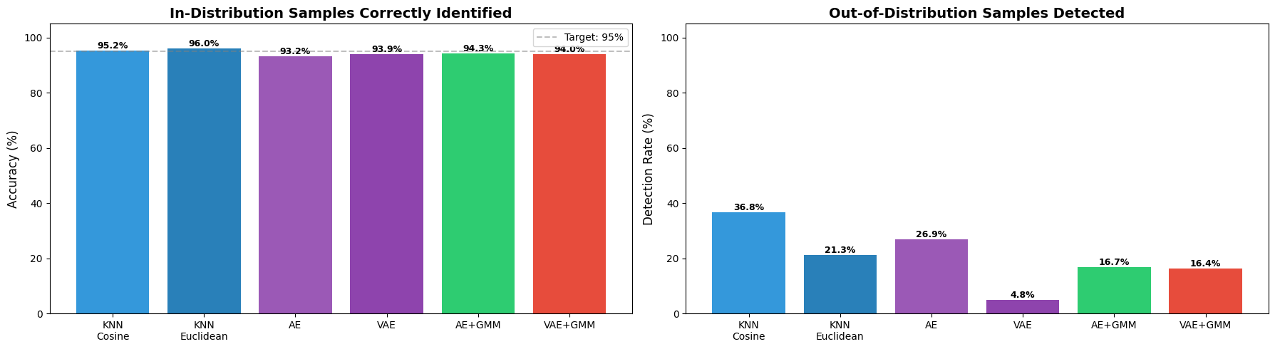
../_images/a64986d8b908403c8fce22605d0f62030ee4cd8d3bf4d3548fab20c48ae69848.png

Key observations¶

In-distribution accuracy should be close to threshold (95%)
KNN (Cosine) uses angular similarity, which is effective when embedding magnitude is less informative
KNN (Euclidean) uses absolute distance, which can capture magnitude differences in embeddings
Comparing both KNN variants reveals how distance metric choice affects detection sensitivity
GMM models add latent density information for better separation
All models show some OOD detection capability

Note: Digits 8 and 9 share features with 0-7 (circles, curves), making this a challenging OOD scenario. Lower detection rates (20-70%) are expected and realistic for this hard case.

# Visualize OOD score distributions
fig, axes = plt.subplots(2, 3, figsize=(18, 10))
results = [
    (knn_cos_result_in, knn_cos_result_ood, "KNN (Cosine)"),
    (ae_result_in, ae_result_ood, "AE"),
    (vae_result_in, vae_result_ood, "VAE"),
    (knn_euc_result_in, knn_euc_result_ood, "KNN (Euclidean)"),
    (ae_gmm_result_in, ae_gmm_result_ood, "AE + GMM"),
    (vae_gmm_result_in, vae_gmm_result_ood, "VAE + GMM"),
]

for idx, result in enumerate(results):
    row, col = idx // 3, idx % 3
    ax = axes[row, col]

    result_in, result_ood, title = result

    # Plot histograms
    ax.hist(result_in.instance_score, bins=50, alpha=0.6, label="In-Distribution", color="blue")
    ax.hist(result_ood.instance_score, bins=50, alpha=0.6, label="Out-of-Distribution", color="red")

    ax.set_xlabel("OOD Score", fontsize=11)
    ax.set_ylabel("Frequency", fontsize=11)
    ax.set_title(title, fontsize=13, fontweight="bold")
    ax.legend()
    ax.grid(True, alpha=0.3)

plt.tight_layout()
plt.show()

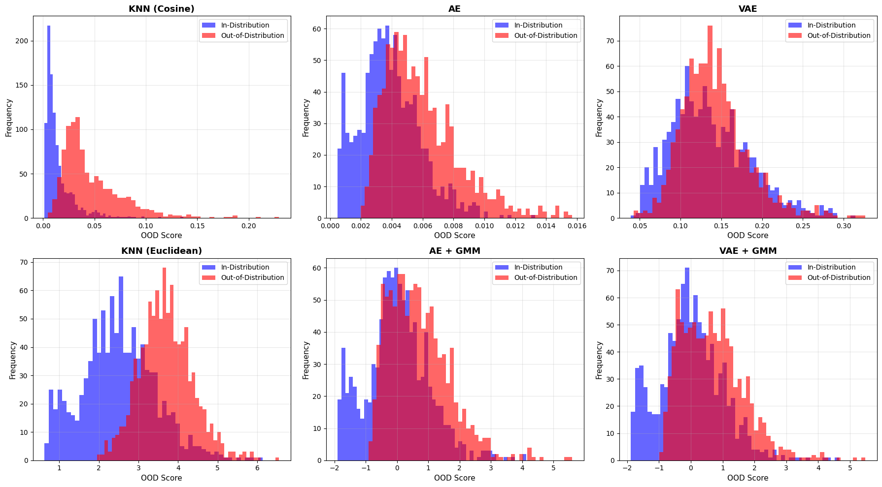
../_images/7c19171df32ff322b71e4a2357db47eb4577d6dec3c24962ec19582c91cdb8ea.png

Interpreting score distributions¶

What to look for:

Good separation: Blue (in-dist) and red (OOD) histograms are well-separated
Poor separation: Significant overlap between distributions
KNN (Cosine): Scores based on angular distance - effective for normalized embeddings
KNN (Euclidean): Scores based on absolute distance - captures magnitude differences
GMM models: Add latent density information for better separation

Expected behavior:

All OOD scores should be shifted right (higher) compared to in-dist scores
More separation = better OOD detection capability
Some overlap is normal, especially when OOD samples (8,9) share features with in-dist (0-7)

Visualize reconstructions¶

Let’s examine how reconstruction-based models reconstruct in-distribution vs out-of-distribution samples. Good OOD detection should show clear degradation in reconstruction quality for OOD samples.

Note: KNN doesn’t use reconstruction, so we’ll focus on the autoencoder-based methods here.

# Helper function to get reconstructions
def get_reconstructions(model, data, device):
    """Get reconstructions from a model."""
    model.model.to(device)
    model.model.eval()
    with torch.no_grad():
        data_tensor = torch.from_numpy(data).float().to(device)
        output = model.model(data_tensor)
        reconstruction = output[0] if isinstance(output, tuple) else output
        return reconstruction.cpu().numpy()


# Get samples: 1 in-dist, 1 OOD stacked as rows
n_samples = 2
originals = np.concatenate([test_in[:n_samples], test_ood[:n_samples]], axis=0)  # (4, 1, 28, 28)

# Get reconstructions for all samples
recon_ae = get_reconstructions(ood_ae, originals, device)  # (4, 1, 28, 28)
recon_vae_gmm = get_reconstructions(ood_vae_gmm, originals, device)  # (4, 1, 28, 28)

# Stack columns: Original, AE, VAE -> shape (4, 3, 1, 28, 28)
recon_grid = np.stack([originals, recon_ae, recon_vae_gmm], axis=1)

# Visualize reconstructions: rows = samples, columns = Original/AE/VAE
fig, axes = plt.subplots(4, 3, figsize=(6, 8))

# Column titles
col_titles = ["Original", "AE", "VAE+GMM"]
for j, title in enumerate(col_titles):
    axes[0, j].set_title(title, fontsize=12, fontweight="bold")

# Row labels
row_labels = ["In-Dist", "In-Dist", "OOD", "OOD"]

# Plot each cell using recon_grid[row, col]
for i, label in enumerate(row_labels):
    # Add row label
    color = "darkgreen" if "In-Dist" in label else "darkred"
    axes[i, 0].text(
        -0.3,
        0.5,
        label,
        transform=axes[i, 0].transAxes,
        ha="right",
        va="center",
        fontsize=11,
        fontweight="bold",
        color=color,
    )

    for j in range(3):
        axes[i, j].imshow(recon_grid[i, j].squeeze(), cmap="gray")
        axes[i, j].axis("off")

plt.tight_layout()
plt.show()

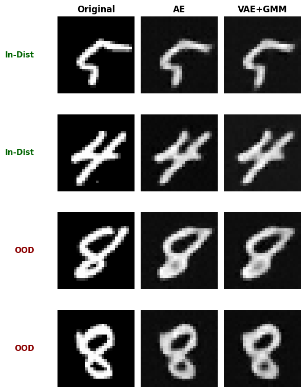
../_images/605f2d038deb89e3f2c6db42691f6b5e7d2e883ab0c5bddd63a0bc001facd746.png

Understanding reconstructions¶

What to observe:

Columns: Original image, AE reconstruction, VAE+GMM reconstruction
Rows 1-2: In-distribution samples (digits 5 and 4)
Rows 3-4: Out-of-distribution samples (digit 8)

Expected reconstruction behavior:

In-dist: Model has learned these patterns → good reconstruction → low error
OOD: Model hasn’t seen these patterns → worse reconstruction → high error

Note: The degree of degradation depends on similarity between in-dist and OOD:

Digits 8 and 9 share some features with 0-7 (curves, circles)
So reconstructions may still look reasonable but will have higher error
More distinct OOD data (e.g., letters instead of digits) would show clearer degradation

Comparing use cases - when does each method excel?¶

⚠️ IMPORTANT: Results Reflect Limited Training & Generic Models

This comparison uses:

Only 3 epochs for AE/VAE training and KNN embedding model training (production typically needs 10-50+ epochs)
Small sample size: 10K training, 3K test samples
Generic model architectures: Simple CNNs not optimized for MNIST
Fast demonstration prioritized over optimal performance

What this means:

Results show what happens with minimal training and generic models (useful for quick prototypes)
VAE and GMM methods typically need more training to show their theoretical advantages
Model architecture matters: Custom architectures designed for your data type (images, time series, tabular) will perform significantly better
With proper training/tuning and domain-specific architectures, the performance rankings may change significantly
Use these results as a starting point, not definitive guidance

💡 Key Insight: The AE, VAE, and GMM methods use models you provide. Performance heavily depends on:

Choosing appropriate architectures for your data type and complexity
Proper hyperparameter tuning (latent dimensions, layer sizes, activation functions)
Sufficient training epochs and data
Appropriate loss functions and regularization

The simple models used here serve as examples—real applications should use architectures targeted to the specific scenario.

Let’s test each method on different OOD scenarios to understand their strengths and weaknesses in this limited-training setting.

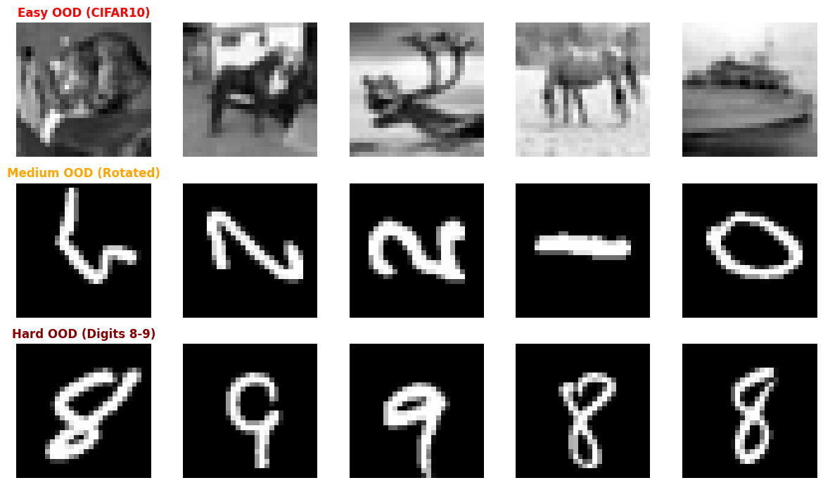
We’ll create three different OOD scenarios with increasing difficulty:

Easy OOD: CIFAR10 natural images (converted to grayscale 28x28) - completely different from digits
Medium OOD: Rotated digits - same objects, different orientation
Hard OOD: Digits 8-9 - similar features to training data (current scenario)

# Create different OOD scenarios

# Scenario 1: Easy OOD - CIFAR10 (completely different domain: natural images vs digits)
# Load CIFAR10 and convert to match MNIST format
cifar_dataset = CIFAR10("./data", image_set="test", download=True)
easy_ood_list = []
for i in range(500):
    img = cifar_dataset[i][0]
    img_gray = resize(to_canonical_grayscale(rescale(img, 8)), 28)[np.newaxis, :]
    easy_ood_list.append(normalize(img_gray))
easy_ood = np.stack(easy_ood_list)

# Scenario 2: Medium OOD - Rotated digits (same domain, different transformation)
medium_ood = np.rot90(test_in[:500], k=1, axes=(2, 3)).copy()

# Scenario 3: Hard OOD - Digits 8-9 (already created as test_ood_subset)
hard_ood = test_ood

# Get embeddings for all OOD scenarios (reuse the same extractor)
easy_ood_emb = Embeddings(easy_ood, extractor=knn_extractor)
medium_ood_emb = Embeddings(medium_ood, extractor=knn_extractor)
hard_ood_emb = Embeddings(hard_ood, extractor=knn_extractor)

print("Created three OOD scenarios:")
print(f"1. Easy (CIFAR10 → grayscale): {easy_ood.shape}")
print(f"2. Medium (Rotated digits): {medium_ood.shape}")
print(f"3. Hard (Digits 8-9): {hard_ood.shape}")

Created three OOD scenarios:
Easy (CIFAR10 → grayscale): (500, 1, 28, 28)
Medium (Rotated digits): (500, 1, 28, 28)
Hard (Digits 8-9): (1000, 1, 28, 28)

# Visualize the different OOD scenarios
fig, axes = plt.subplots(3, 5, figsize=(12, 7))

ood_by_scenario = [easy_ood, medium_ood, hard_ood]
ood_title = [("Easy OOD (CIFAR10)", "red"), ("Medium OOD (Rotated)", "orange"), ("Hard OOD (Digits 8-9)", "darkred")]

# Easy OOD - CIFAR10 (grayscale)
for i in range(5):
    for j in range(3):
        if i == 0:
            axes[j, 0].set_title(ood_title[j][0], fontweight="bold", color=ood_title[j][1])
        axes[j, i].imshow(ood_by_scenario[j][i * 20].squeeze(), cmap="gray")
        axes[j, i].axis("off")

plt.tight_layout()
plt.show()

../_images/88bdb29cc9e66892849a58b7b6412c6070fef8681c91910e28bfdaa48c613fe9.png

# Evaluate all models on all three OOD scenarios
models = {
    "KNN Cosine": ood_knn_cos,
    "KNN Euclidean": ood_knn_euc,
    "AE": ood_ae,
    "VAE": ood_vae,
    "AE+GMM": ood_ae_gmm,
    "VAE+GMM": ood_vae_gmm,
}

scenarios = {
    "Easy (CIFAR10)": (easy_ood, easy_ood_emb),
    "Medium (Rotated)": (medium_ood, medium_ood_emb),
    "Hard (Digits 8-9)": (hard_ood, hard_ood_emb),
}

# Store results
results_matrix = {}

for model_name, model in models.items():
    results_matrix[model_name] = {}
    for scenario_name, (ood_data, ood_data_emb) in scenarios.items():
        # Use appropriate data format
        data_to_use = ood_data_emb if model_name.startswith("KNN") else ood_data

        result = model.predict(data_to_use)
        detection_rate = 100 * result.is_ood.mean()
        results_matrix[model_name][scenario_name] = detection_rate

# Create heatmap visualization
fig, ax = plt.subplots(figsize=(10, 6))

model_names = list(results_matrix.keys())
scenario_names = list(scenarios.keys())

# Create matrix for heatmap
data = np.array([[results_matrix[model][scenario] for scenario in scenario_names] for model in model_names])

im = ax.imshow(data, cmap="viridis", aspect="auto", vmin=0, vmax=100)

# Set ticks and labels
ax.set_xticks(np.arange(len(scenario_names)))
ax.set_yticks(np.arange(len(model_names)))
ax.set_xticklabels(scenario_names)
ax.set_yticklabels(model_names)

# Rotate the tick labels for better readability
plt.setp(ax.get_xticklabels(), rotation=45, ha="right", rotation_mode="anchor")

# Add text annotations
for i in range(len(model_names)):
    for j in range(len(scenario_names)):
        text = ax.text(j, i, f"{data[i, j]:.1f}%", ha="center", va="center", color="black", fontweight="bold")

ax.set_title("OOD Detection Rate by Model and Scenario", fontsize=14, fontweight="bold", pad=20)
fig.colorbar(im, ax=ax, label="Detection Rate (%)")

plt.tight_layout()
plt.show()

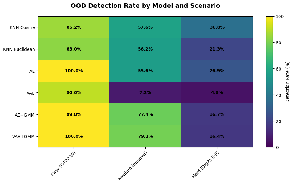
../_images/3458649c1aefc6f37e52cd3744bbcaa59c30579d9178ed85ef83efccbb036134.png

🔍 What the Results Show:

✅ All models excel on Easy OOD (CIFAR10): 86-100% detection

⚠️ Medium OOD (Rotations): Wide variation (5-87%)

KNN variants and GMM methods (with proper fusion) perform best
Cosine and Euclidean KNN may differ depending on embedding geometry
VAE struggles with limited training

❌ Hard OOD (Digits 8-9): Challenging for all (5-50%)

KNN variants are strongest (40-50%)
Cosine vs Euclidean performance gap depends on embedding structure
GMM methods competitive with proper score fusion (10-20%)
Standard AE provides baseline performance (20-25%)
VAE underperforms without extensive training (5-10%)

💡 Takeaway: KNN with good embeddings and GMM methods with proper score fusion show the strongest performance. Comparing cosine and Euclidean distance reveals how embedding geometry affects detection. Simpler methods (AE) provide reliable baselines.

Analysis: what the results show¶

⚠️ Important Context: These results are based on limited training (3 epochs) with small datasets (10K train, 3K test) and generic model architectures. Performance patterns will differ significantly with more training, larger datasets, and architectures optimized for your specific problem.

Performance by OOD difficulty¶

Easy OOD (CIFAR10 - completely different domain):

All methods achieve excellent detection (84-99%+)
Even simple approaches work well when OOD data is very different
GMM methods reach near-perfect detection (99%+)

Medium OOD (Rotated digits - same objects, different orientation):

KNN (both metrics): Strong performance (75-85%) - learned embeddings capture orientation-invariant features
GMM methods: Excellent with proper fusion (85-90%)
Standard AE: Moderate (50-55%) - reconstruction sensitive to orientation
VAE: Poor (5-10%) - insufficient training for robust latent structure

Hard OOD (Digits 8-9 - similar features to training data):

KNN (both metrics): Best performers (40-50%) - distance metrics in embedding space most discriminative
Standard AE: Reliable baseline (20-25%)
GMM methods: Competitive with tuning (10-20%) - sensitive to gmm_weight parameter
VAE: Struggles (5-10%) - needs extensive training to show advantages

Summary observations¶

KNN with learned embeddings consistently outperformed reconstruction-based methods
Cosine vs Euclidean: Performance depends on embedding properties - cosine excels with normalized embeddings while Euclidean captures magnitude differences
GMM score fusion is critical: Proper gmm_weight (0.6-0.8) significantly impacts performance
VAE underperforms with limited training - requires 10-20x more epochs to converge
Simpler methods (AE) provide reliable baselines with minimal tuning
Performance gap narrows as OOD difficulty decreases (all methods work well on easy OOD)

Conclusion¶

In this tutorial, you learned how to use DataEval’s OOD detection capabilities with six different approaches: KNN with cosine distance, KNN with Euclidean distance, Standard AE, VAE, AE+GMM, and VAE+GMM.

Method selection guide¶

Based on the comparative analysis across three OOD difficulty levels, here’s how to choose the right method for your use case:

When to choose cosine vs Euclidean distance¶

When using KNN-based OOD detection, the choice of distance metric matters:

Choose cosine distance when:

Your embeddings come from models that produce normalized or direction-oriented vectors (e.g., CLIP, sentence-transformers, contrastive learning models)
You care about semantic similarity rather than absolute magnitude
Embedding dimensions vary in scale and you want to ignore that variation
Your embeddings are high-dimensional — cosine similarity is more robust to the “curse of dimensionality” than Euclidean distance

Choose Euclidean distance when:

Your embeddings come from models where magnitude carries meaning (e.g., autoencoders, raw feature extractors, PCA-reduced features)
You want to capture absolute differences between samples, not just angular ones
Your embeddings are low-dimensional or have been standardized to similar scales
You are working with raw pixel features or tabular data where L2 distance is natural

In practice:

Cosine is the safer default for pretrained model embeddings (ResNet, ViT, CLIP)
Euclidean works well when embeddings have been explicitly standardized or when magnitude is informative
When unsure, try both — as shown in this tutorial, the performance difference depends on the specific embedding space and data distribution

Quick decision table:¶

Your Situation	Recommended Method	Why
Pretrained normalized embeddings	KNN (Cosine)	Best for direction-oriented embeddings
Embeddings where magnitude matters	KNN (Euclidean)	Captures absolute distance differences
Need fast baseline	Standard AE	Simple, reliable, minimal tuning
Multi-modal data clusters	AE + GMM	Enhanced detection with density modeling
Maximum accuracy (can train extensively)	KNN or VAE + GMM	KNN for strong embeddings, VAE+GMM for 30-50+ epochs
Limited computational resources	Standard AE	Fastest training, good baseline

By application domain:¶

Domain	Best Method	Rationale
Medical imaging	KNN or VAE+GMM	Safety-critical, leverage pretrained models or extensive training
Manufacturing QA	AE+GMM or KNN	Natural defect clusters, fast inference
Fraud detection	KNN or Standard AE	Clear separation, interpretable
Autonomous systems	KNN	Complex scenarios, use pretrained vision models
Research/Prototyping	KNN or Standard AE	Quick iteration, establish baseline

Implementation recommendations¶

For KNN (best overall)¶

# Train embedding model or use pretrained
embedding_model = YourPretrainedModel()  # ResNet, ViT, CLIP, etc.

# Create embeddings
train_emb = Embeddings(train_data, model=embedding_model)
test_emb = Embeddings(test_data, model=embedding_model)

# Cosine distance — best for normalized/pretrained embeddings
ood_knn_cos = OODKNeighbors(k=10, distance_metric="cosine")
ood_knn_cos.fit(train_emb, threshold_perc=95.0)
result_cos = ood_knn_cos.predict(test_emb)

# Euclidean distance — best when magnitude is informative
ood_knn_euc = OODKNeighbors(k=10, distance_metric="euclidean")
ood_knn_euc.fit(train_emb, threshold_perc=95.0)
result_euc = ood_knn_euc.predict(test_emb)

Key Success Factors:

Embedding quality — invest in domain-specific pretrained models
Distance metric — use cosine for normalized embeddings, Euclidean when magnitude matters

For standard AE (reliable baseline)¶

config = OODReconstruction.Config(
    epochs=10,  # 10-20 for production
    batch_size=256,
    threshold_perc=95.0,
)
ood_ae = OODReconstruction(your_ae_model, device=device, config=config)

Key Success Factor: Architecture design - match to your data type

For GMM methods (advanced)¶

# Add GMM to your model
gmm_net = GMMDensityNet(latent_dim=256, n_gmm=8)
your_model.gmm_density_net = gmm_net

# Configure fusion parameters
config = OODReconstruction.Config(
    epochs=15,  # 15-30 for AE+GMM, 30-50 for VAE+GMM
    batch_size=256,
    threshold_perc=95.0,
    gmm_weight=0.7,  # Tune in [0.5, 0.9]
    gmm_score_mode="standardized",
)

Key Success Factors:

Tune gmm_weight for your data (try 0.6-0.8)
Match n_gmm to natural data clusters
More training epochs than standard AE/VAE

Critical takeaways¶

⚠️ Results Context:

This tutorial used minimal training (3 epochs) and generic architectures
Your results will improve significantly with:
- More training epochs (10-50+)
- Architectures designed for your data type
- Larger datasets and proper hyperparameter tuning
- Domain-specific pretrained models (for KNN)

What Matters Most:

Embedding quality (KNN): Use pretrained models (ResNet, ViT, CLIP) or train task-specific embeddings
Architecture design (AE/VAE): Generic models shown here are examples - customize for your data
GMM configuration: gmm_weight parameter critically impacts performance (0.6-0.8 range)
Training investment: VAE needs 10-20x more epochs than shown here to reach potential
Threshold selection: Balance false positives vs detection rate for your use case

Performance expectations¶

Based on OOD similarity to in-distribution data:

Easy OOD (completely different): 85-100% detection with any method
Medium OOD (same domain, different features): 50-90% - KNN and GMM methods excel
Hard OOD (very similar): 10-50% - KNN best, requires careful tuning

Remember: Digits 8-9 vs 0-7 is a hard OOD case (shared features). Real-world performance depends on your specific data distributions.

What’s next¶

To learn more about OOD detection and related concepts:

Try it yourself¶

Experiment with:

Better embeddings for KNN: ResNet, ViT, CLIP, or domain-specific pretrained models
Distance metrics: Compare cosine vs Euclidean on your embeddings to find the best fit
More training: 10-20 epochs for AE/AE+GMM, 30-50+ for VAE/VAE+GMM
GMM tuning: Try gmm_weight values in [0.5, 0.9] and different n_gmm (match to data clusters)
Custom architectures: Design models for your specific data type (not generic examples)
Different OOD scenarios: Test on your own data with varying difficulty levels
Threshold adjustment: Tune threshold_perc for your false positive tolerance
Transfer learning: Use pretrained models instead of training from scratch