Glossary
A
- Accuracy
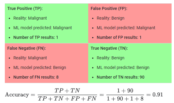
A metric for evaluating classification models based on the fraction of predictions our model got correct. Mathematically, accuracy has the following definition:
\(Accuracy = \frac{\text{Number of correct predictions}}{\text{Total number of predictions}}\)
For Binary Classification, it is defined as the following:
\(Accuracy = \frac{(TP + TN)}{(TP + TN + FP + FN)}\)
where:
A binary example with benign and malignant tumor detection rates is shown in the following image:
- Anderson-Darling Test
A non-parametric statistical test for comparing distributions that places greater weight on differences in the tails compared to tests like the Kolmogorov-Smirnov (K-S) test or Cramér-von Mises (CVM) Test. The Anderson-Darling test measures weighted squared differences between two empirical cumulative distribution functions, with its weighting function emphasizing discrepancies at the distribution extremes. This makes it particularly powerful for detecting drift in heavy-tailed distributions or scenarios where tail behavior is critical, such as in safety-critical computer vision applications where rare edge cases (extreme lighting conditions, unusual object poses) must be detected. The test is commonly used in quality control and reliability engineering, and in the context of machine learning, it serves as a sensitive method for identifying distributional shifts that might indicate model degradation.
- Artificial Intelligence (AI)
Artificial Intelligence, or AI, is technology that enables computers and machines to simulate human intelligence and problem-solving capabilities. It is modeled after the decision-making processes of the human brain that can ‘learn’ from available data and make increasingly more accurate classifications or predictions over time. For the applications in DataEval, Neural Networks are the main modeling method.
See Neural Network
- Aspect Ratio
For Images, the ratio of the width (in pixels) over the height (in pixels)
\(Aspect Ratio = \frac{width}{height}\)
See Image Size
- AUROC
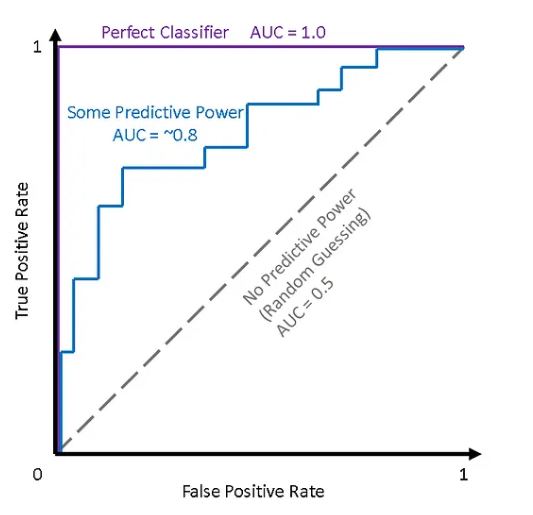
The Area Under the ROC Curve (AUROC) is a metric that measures the performance of a classification model at all possible classification thresholds. It’s calculated by measuring the two-dimensional area underneath a ROC curve from (0,0) to (1,1). AUROC can range from 0 to 1, with higher values indicating better performance:
An example scale might be:
0: A perfectly inaccurate test
0.1-0.4: Unacceptable. Inaccurate a majority of the time
0.5: A random model or no discrimination
0.6: Unacceptable. Low discrimination
0.7–0.8: Acceptable
0.8–0.9: Excellent
1: A perfect model that can correctly distinguish between all positive and negative class points
- Autoencoder
An autoencoder is a type of artificial neural network that learns efficient encodings of unlabeled data by doing unsupervised learning. An autoencoder learns two functions: an encoding function that transforms the input data into a latent space, and a decoding function that recreates the input data from the encoded representation. Typically used for dimensionality reduction.
- Average Pooling
A type of pooling layer that calculates the average value from a group of pixel values produced by a convolutional layer. Typically used in a convolutional neural network to reduce the dimensionality between layers.
B
- Balance
A measure of co-occurrence of metadata factors with class labels. Metadata factors that spuriously correlate with individual classes may allow a model to learn shortcut relationships rather than the salient properties of each class.
- Baumgartner-Weiss-Schindler Test
A modern non-parametric statistical test for comparing two distributions. The Baumgartner-Weiss-Schindler (BWS) test combines advantages of several classical tests and has particularly high statistical power for detecting distributional differences. It has strong sensitivity to tail differences similar to the Anderson-Darling test while also being effective at detecting location and scale shifts. In the context of drift detection, BWS is recommended for critical applications where missing drift is costly, such as production computer vision systems in medical imaging or autonomous driving.
- Bayes Error Rate (BER)
In statistical classification, bayes error rate is the lowest possible error rate for any classifier of a random outcome (into, for example, one of two categories) and is analogous to the irreducible error. A number of approaches to the estimation of the bayes error rate exist. In general, it is impossible to compute the exact value of the bayes error.
- Bias
The systematic error or deviation in a model’s predictions from the actual outcomes. Bias can arise from various sources, such as a skewed or imbalanced dataset, incomplete feature representation, or the use of biased algorithms.
- Binary Classification
Binary classification is a fundamental task in machine learning, where the goal is to categorize data into one of two classes or categories.
- Black-box Shift Estimation (BBSE)
A method for measuring label shift on machine learning datasets. It is calculated using a confusion matrix and only requires that the matrix be invertible. It calculates the probability of a label l in the target dataset over the probability of the same label in the test data set. \((W = \frac{q(y)}{p(y)})\) It is solved as a linear equation \(Ax = b\) where A is the Confusion Matrix estimated on the training dataset and b is average output of the predictor function calculated on the target dataset.
- Blur
For Images, the loss of sharpness resulting from motion of the subject or the camera during exposure. Objects appear less clear or distinct. It is calculated using the variance on a Laplacian filter. A low value on the variance indicates very few sharp edges which points toward a blurry image.
- Bonferroni Correction
The Bonferroni Correction is a multiple-comparison correction used when several dependent or independent statistical tests are being performed simultaneously. The reason is that while a given alpha value may be appropriate for each individual comparison, it is not appropriate for the set of all comparisons.
- Brightness
For images, brightness is a measure of how light or dark an image is overall, or its luminous intensity after it’s been digitized or acquired by a camera. It can also be described as the relative intensity of a visible light source’s energy output.
C
- Categorical Variable
In statistics, a categorical variable (also called qualitative variable) is a variable that can take on one of a limited, and usually fixed, number of possible values, assigning each individual or other unit of observation to a particular group or nominal category on the basis of some qualitative property.
- Channel (Images)
Descriptive component of an image. For example, gray-scale images have one channel describing brightness levels, while red-green-blue (RGB) images have 3 channels describing the red, green, blue brightness levels.
- Chi-Square Test of Independence
The Chi-Square Test of Independence determines whether there is an association between Categorical Variables (i.e., whether the variables are independent or related). For more information on how to compute see the following explanation: Chi Square Test Of Independence
- Classification
Classification is a supervised machine learning method where the model tries to predict the correct label of a given input data value. For instance, an algorithm can learn to predict whether a given email is spam or ham (no spam) or whether an image contains a house or a car.
- Cluster Analysis
Cluster Analysis is a statistical method for processing data. It is primarily used in classification projects. It works by organizing items into groups, or clusters, based upon how closely associated they are. The objective of cluster analysis is to find similar groups of subjects, where the “similarity” between each pair of subjects represents a unique characteristic of the group vs. the larger population/sample. It is an unsupervised learning algorithm, meaning the number of clusters is unknown before running the model.
- Completeness
Completeness informs users the degree to which images span the learned embedding space. A complete dataset is one which contains every combination of latent variable ranges.
Completenessquantifies the extant to which a dataset is complete.See, diversity,balance,parity, and coverage for related metrics.
- Concept Drift
Concept drift is a specific kind of data drift where there is a change in the relationship between the input data and the model target. It reflects the evolution of the underlying problem statement or process over time.
- Confidence Level
In statistics, the confidence level indicates the probability with which the estimation of the location of a statistical parameter (for example an arithmetic mean) in a sample survey is also true for the actual population.
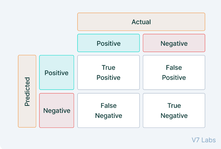
- Confusion Matrix
A matrix made up of the following measurements: True Positives, True Negatives, False Positives and False Negatives. An image is shown below.
See True Positive Rate (TP), True Negative Rate (TN), False Positive Rate (FP), False Negative Rate (FN)
- Contractive Autoencoder (CAE)
A type of autoencoder which is designed to be sensitive to small changes in the training dataset. It attempts to increase the robustness of the model by emphasizing the accurate encoding of small changes in the training data.
- Convolutional Layer
Input layer to a convolutional neural network. Core building block of CNN where a majority of the computation occurs. It requires 3 components; input data, a filter or kernel (matrix), and a feature map. The kernel sweeps across the input data’s feature map using a dot product operation to ‘find’ the features. This process is called convolution.
- Convolutional Neural Network (CNN)
A type of Deep Neural Network used in computer vision applications such as image classification, image segmentation and image and video recognition. It uses at a minimum of 3 layers; the convolutional layer, the pooling layer and the Fully Connected (FC) Layer. With each layer, the CNN increases its complexity, identifying greater portions of the input image.
- Coverage
A measure of the distribution of the images in a dataset. A covered dataset has at least one image for every distinguishing property of the data set.
- Covariate Shift
A type of drift where the distribution of input features changes between training and deployment, while the relationship between inputs and outputs remains the same.
- Cramér-von Mises (CVM) Test
The Cramér-von Mises algorithm tests the null hypothesis that a data sample (i.e. operational dataset) comes from a pre-specified population distribution or a family of such distributions with the idea that if the operational dataset does not come from the same distribution or family of distributions as the training dataset then data drift may have occurred. It is similar to the Kolmogorov-Smirnov test.
- Cross-Validation
A technique for assessing model performance by splitting data into folds.
D
- Dataset Splits
Dataset splits, also known as data splitting, is the process of dividing a data set into multiple subsets to help train, test and evaluate machine learning models.
- Deduplication
The process of identifying and exact or extremely similar data or images from a data set. A near duplicate is defined as within one standard deviation of the relevant distance statistic within a cluster of a data point in a data set.
- Deep Neural Network (DNN)
A deep neural network is an artificial neural network with multiple layers between the input and output layers. There are different types of neural networks but they generally consist of the same components: weights, biases, and activation function (and corresponding locations in the network). These components, as a whole, mimic the functionality of the human brain.
- Denoising Autoencoder (DAE)
A type of autoencoder which is designed to increase its robustness by stochastically training the model for the reconstruction phase rather than the encoding phase.
- Developmental Dataset
Dataset used in for machine learning model development. It consists of several dataset splits that can include training, validation and testing splits.
- Dimensionality Reduction
Dimensionality reduction is a method for representing a given dataset using a lower number of features (i.e. dimensions) while still capturing the original data’s meaningful properties. This amounts to removing irrelevant or redundant features, or simply noisy data, or combining features into a reduced number of new features to create a model with a lower number of variables.
- Divergence
Divergence is a kind of statistical distance: a function which establishes the separation from one probability distribution to another on a statistical manifold.
- Diversity
A measure of the distribution of metadata factors in the dataset. A balanced dataset has an even distribution of class labels and generative factors.
- Domain Classifier (DC)
A machine learning model that attempts to distinguish between two datasets.
- Drift
In predictive analytics, data science, machine learning and related fields, the phenomenon where the statistical properties of the data change over time. It occurs when the underlying distribution of the input features or the target variable (what the model is trying to predict) shifts, leading to a discrepancy between the training data and the real-world data the model encounters during deployment.
- Duplicates
Statistical duplicates, or duplicate data, are repeated records or observations in a dataset. They can be caused by human error, technical errors, and/or data manipulation. In the case of DataEval for the image classification and/or detection tasks, exact matches are found using a byte hash of the image information, while near matches use a perception-based hash
E
- Embeddings
A compact, fixed-length vector representation of an image (or other data object) produced by passing it through a trained neural network. The network discards pixel-level detail and encodes the semantic or structural content that the network learned to distinguish during training. Images that are similar in the sense the network was trained for will be close together in the embedding space; images that are dissimilar will be far apart.
Why DataEval uses embeddings. Many DataEval evaluators — including coverage, completeness, Prioritize, DriftKNeighbors, OODKNeighbors, and label_errors — operate on embeddings rather than raw images, because geometric distance in embedding space is a meaningful proxy for semantic similarity. Outlier detection and duplicate detection can also use embeddings as a third detection mode alongside image-statistics-based methods.
What makes a good embedding for DataEval. The right embedding depends on what the evaluators need to measure:
Coverage and completeness require that the embedding reflects the variation that matters operationally — scene content, target type, background, imaging conditions. Self-supervised models (DINO, SimCLR, CLIP) trained on large natural-image corpora are appropriate for general natural imagery but may fail to encode operationally relevant variation in specialized domains (sonar, synthetic aperture radar, infrared).
Duplicate and outlier detection (cluster mode) require that the embedding separates genuinely different images. Embeddings that collapse variation — mapping very different images to nearby vectors — will produce clusters that do not align with meaningful semantic groupings.
Label error detection requires that the embedding separates classes. If a model trained on natural images is applied to a dataset with fine-grained military vehicle categories, self-supervised embeddings may not separate those categories well. In this case, a supervised embedding trained on the target classes — or a model fine-tuned on domain data — will produce more meaningful intra/extra class distances.
Drift and OOD detection in embedding space require that the embedding is sensitive to the kind of change being monitored. A model trained on classification will encode class-discriminative features; it may be insensitive to background or sensor changes that do not affect class predictions. A self-supervised model may capture those environmental changes more directly.
Supervised vs. self-supervised. Supervised embeddings (from a model trained to classify or detect) encode class-discriminative features well but may suppress variation that is not class-relevant. Self-supervised embeddings (from contrastive or masked-image-modeling objectives) encode a broader range of visual features but without specific sensitivity to any particular task. For highly imbalanced or rare-class datasets, self-supervised embeddings may embed the rare class poorly because the dominant background signal overwhelms small target signatures; in that case, a supervised model is preferable.
Domain match. A model trained on ImageNet produces meaningful embeddings for natural photographic images but may produce arbitrary or degenerate embeddings for out-of-domain data (medical imagery, aerial infrared, sonar). Embeddings should be validated for the target domain before being used as input to any DataEval evaluator. A practical check: verify that images you expect to be similar are close in the embedding space and that images you expect to be different are far apart.
Dimensionality. Most DataEval evaluators work best with embeddings below 500 dimensions. High-dimensional embeddings suffer from the curse of dimensionality: distances become increasingly uniform, making nearest-neighbor and cluster-based methods unreliable. Standard feature extractor outputs (ResNet, ViT, CLIP image encoder) typically produce 512–2048 dimensional vectors; applying PCA or another dimensionality reduction step before running coverage, clustering, or prioritization is advisable when dimension exceeds 500.
See also: :term:
Feature Extractor, :term:Out-of-Distribution (OOD)- Entropy
Entropy is a measure of how evenly data examples are distributed over their set of possible values. If all possible values are equally likely, then entropy is maximal. If only one value ever occurs, entropy is zero. Entropy is used to evaluate feature importance, measure dataset complexity, and detect drift in data distributions over time.
- Epoch
Each time a dataset passes through an algorithm, it is said to have completed an epoch. Therefore, epoch, in machine learning, refers to one entire pass of training data through the algorithm.
F
- F1-Score
One way to capture the precision-recall curve in a single metric. F1-Score combines precision and recall scores with equal weight, and works also for cases where the datasets are imbalanced as it requires both precision and recall to have a reasonable value. It is the harmonic mean of precision and recall and has a range of [0-1]. It is defined as follows:
\(F1 = 2* \frac{\text{( Precision * Recall)}}{\text{(Precision + Recall)}}\)
- False Discovery Rate (FDR)
The FDR is defined as the ratio of the number of False Positive Rate (FP) classifications (false discoveries) to the total number of True Positive Rate (TP) classifications (rejections of the null).
\(FDR = \frac{FP}{(FP + TP)}\)
where:
- False Discovery Rate (FDR) Correction
False Discovery Rate Correction is a statistical procedure for correcting for the problem caused by running multiple hypothesis tests at once. It is typically used in high-throughput experiments in order to correct for random events that falsely appear significant.
- False Negative Rate (FN)
A measure of machine learning model accuracy. It measures the frequency at which a negative prediction was found for a positive ground truth value.
See Confusion Matrix
- False Positive Rate (FP)
A measure of machine learning model accuracy. It measures the frequency at which a positive prediction was found for a negative ground truth value.
See Confusion Matrix
- FB Score
F “Beta” Score: The F-beta score is the weighted harmonic mean of precision and recall with a range of 0 (worst) to 1 (best). The beta (\(\beta\)) parameter represents the ratio of the recall importance to precision importance. A value greater than 1 gives more weight to recall while a value less than 1 favors precision. The formula is shown below:
\(F_\beta =\frac{(1 +\beta^2)TP}{(1 +\beta^2)TP + FP + \beta^2FN}\)
where:
- Feasibility
Feasibility is a measure of whether the available data (both quantity and quality) can be used to satisfy the necessary performance characteristics of the machine learning model.
- Feature Extractor
A neural network, or the encoder portion of one, used to transform raw input data into an :term:
embedding— a compact vector representation suitable for downstream analysis. The network is run in inference mode only; its weights are not updated during DataEval’s evaluation process.In DataEval, a feature extractor is any callable that accepts an image (or batch of images) and returns a fixed-length vector. This includes full classification networks with the final classification layer removed, dedicated encoder architectures (ResNet, ViT, DINO), and multimodal encoders such as the image encoder from CLIP. DataEval provides lightweight built-in extractors for common cases and accepts any MAITE-compliant extractor via the
Encoderprotocol.The choice of feature extractor is the single most consequential decision when using any embedding-dependent evaluator. A well-chosen extractor makes geometric distance in the output space meaningful for the task at hand; a poorly chosen one produces distances that are arbitrary relative to the analysis goal. See :term:
Embeddingsfor guidance on extractor selection.- Fully-Connected Layer
Layer in a neural network. Every node in the layer is connected to every node in the previous layer. It performs the task of classification by creating probabilities that input data contains the features filtered for by the neural network.
G
- Generative Model
A type of machine learning model which can generate new data that is similar to the input/training data for the model. For example, large language models (LLMs) are able to generate new text from their large pool of language data.
H
- Hamming Distance
The Hamming Distance between two strings of equal length is the number of positions at which these strings vary. In more technical terms, it is a measure of the minimum number of changes required to turn one string into the other. In DataEval, images are turned (hashed) into strings in order to compute their Hamming Distance.
- Hilbert Space
A Hilbert Space is an inner product space that is a complete space where distance between instances can be measured with respect to the norm or distance function induced by the inner product. The Hilbert Space generalizes the Euclidean space to a finite or infinite dimensional space. Usually, the Hilbert Space is high dimensional. By convention in machine learning, unless otherwise stated, Hilbert space is also referred to as the feature space.
I
- Image Size
The total number of pixels in an image. It is the product of the width (in pixels) and height (in pixels).
\(Image Size = width*height\)
- Inference
Statistical inference is a method of making decisions about the parameters of a population, based on random sampling.
- Irreducible Error
The irreducible error, also known as noise, represents the variability or randomness in the data that cannot be explained by a regression model. The irreducible error arises from various sources such as unmeasured variables, measurement errors, or natural variability in the target variable. It is independent of the predictor variables X and cannot be reduced by improving the model. The only way to reduce irreducible error is by improving the quality of the data or acquiring additional information that captures the unexplained variability.
J
- Joint Sample
A joint sample is a draw from the underlying distribution of both input data and its (potentially unknown) corresponding label. The correlation between input data and matching label is what a model attempts to capture. The joint distribution from which the joint sample is drawn characterizes this correlation.
K
- Kolmogorov-Smirnov (K-S) test
In statistics, the Kolmogorov–Smirnov Test is a nonparametric test of the equality of continuous, one-dimensional probability distributions that can be used to test whether a sample came from a given reference probability distribution (one-sample K–S test), or to test whether two samples came from the same distribution (two-sample K–S test). Intuitively, the test provides a method to qualitatively answer the question “How likely is it that we would see a collection of samples like this if they were drawn from that probability distribution?” or, in the second case, “How likely is it that we would see two sets of samples like this if they were drawn from the same (but unknown) probability distribution?”. It is named after Andrey Kolmogorov and Nikolai Smirnov.
L
- Label Parity
Label parity is a means for assessing equivalence in label frequency between datasets. Label parity informs the user if the distribution of labels is different.
- Label Shift
In many real-world applications, the target (testing) distribution of a model can differ from the source (training) distribution. Label shift arises when class proportions differ between the source and target, but the feature distributions of each class do not. For example, the problems of bird identification in San Francisco (SF) versus New York (NY) exhibit label shift. While the likelihood of observing a snowy owl may differ, snowy owls should look similar in New York and San Francisco.
- Laplacian Filter
The Laplacian filter is an edge detection filter. It uses the second derivatives of an image to find regions of rapid intensity change.
- Latent Space
Also known as a Latent Feature Space or Encoded Space, is an embedding of a set of items within a manifold in which items resembling each other under some encoding are positioned close to one another. Positions are defined by a set of latent variables that emerge from the properties of the objects. For example, placing images within a Gaussian Distribution based upon their color properties defines the parameters of the Gaussian and reduces the number of parameters for the images.
- Linter
The data linter identifies potential issues (lints) in the ML training data. The term “linter” stems from the origins of a tool known as “lint,” which was initially developed by Stephen C. Johnson in 1978 at Bell Labs. For DataEval and imagery, it identifies issues such as image quality (overly bright/dark, overly blurry, lacking information), unusual image properties (shape,size, *channels), as well as duplicates and outliers.
M
- Machine Learning (ML)
Machine learning (ML) is a branch of artificial intelligence and computer science that focuses on the using data and algorithms to enable AI to imitate the way that humans learn, gradually improving its accuracy. In general, machine learning algorithms are used to make a prediction or classification. Based on some input data, which can be labeled or unlabeled, your algorithm will produce an estimate about a pattern in the data.
- Manifold
In mathematics, a manifold is a topological space that locally resembles Euclidean space near each point. One dimensional manifolds include lines and circles. Two dimensional manifolds are also called surfaces. One example is the family of Gaussian or Normal Functions. They form a manifold parameterized by the expected value and variance of the Gaussian functions.
- Mann-Whitney U Test
A non-parametric statistical test (also known as the Wilcoxon rank-sum test) that compares whether two samples come from the same distribution by analyzing their ranks rather than their raw values. The Mann-Whitney U test is particularly robust to outliers and extreme values because it uses rank-based comparisons. It is most sensitive to shifts in the median (location shifts) and makes minimal assumptions about the underlying distributions, requiring only that the data be ordinal (rankable). In the context of drift detection in computer vision, it is especially useful for image quality metrics that may contain noise spikes or for outdoor vision systems with weather-induced variance and illumination extremes.
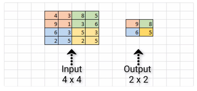
- Maximum Pooling
Method used in the pooling layer of a convolutional neural netwok. It uses the maximum value in a group of pixel values (typically a 2 x 2 or 3 x 3 area) produced from the convolutional layer to reduce the dimensionality of the result. An image of the operation is shown below.
- Maximum Mean Discrepancy (MMD) Drift Detection
MMD Drift Detection is a method which compares the mean embeddings of each sample: A reference sample and a target sample. For example, one might use the mean image embedding for a set of training data, and compare that to the mean embedding of an operational dataset. If the two means are significantly different from one another, drift is detected. What constitutes a “significant” difference stems from underlying assumptions about the distribution of embeddings. More info can be found here: MMD Reference Paper.
See Drift
- Mean Average Precision
A measure to evaluate the performance of object detection and segmentation systems over all classes covered by the system. It is calculated using the confusion matrix, precision and recall metrics and the Area Under the Curve (AUC) metric. It is the average precision for each class averaged over the number of classes.
- Minimum Pooling
Method used in the pooling layer of a convolutinal neural network. It uses the minimum value in a group of pixel values (typically a 2 x 2 or 3 x 3 area) produced from the convolutional layer to reduce the dimensionality of the result.
- Modular AI Trustworthy Engineering (MAITE)
A toolbox of common types, protocols (a.k.a. structural subtypes) and tooling to support AI test and evaluation (T&E) workflows. Part of the Joint AI T&E Infrastructure Capability (JATIC) program. Its goal is to streamline the development of JATIC Python projects by ensuring seamless, synergistic workflows when working with MAITE-conforming Python packages for different T&E tasks.
- Mutual Information (MI)
In probability theory and information theory, the mutual information of two random variables is a measure of the mutual dependence between the two variables. More specifically, it quantifies the “amount of information” obtained about one random variable by observing the other random variable.
N
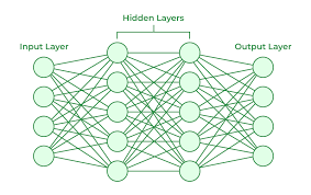
- Neural Network
A neural network is a method in artificial intelligence that teaches computers to process data in a way that is inspired by the human brain. An example depiction is shown below:
- Null Hypothesis
In scientific research, the null hypothesis (often denoted H0) is the claim that the effect being studied does not exist. The null hypothesis can also be described as the hypothesis in which no relationship exists between the two sets of data or variables being analyzed. If the null hypothesis is true, any experimentally observed effect is due to chance alone, hence the term “null”.
- NumPy
NumPy is a Python Library used for working with arrays. It also has functions for working in linear algebra, fourier transforms and matrices (used in convolution). NumPy was created in 2005 by Travis Oliphant.
O
- Object Detection
Object Detection is a computer vision technique for locating instances of objects in images or videos. Object detection algorithms typically leverage machine learning or deep learning to produce meaningful results.
- Operational Dataset
Dataset used while a machine learning model is in operation and not used or seen during training. It may or may not match the characteristics of the developmental dataset.
See Drift.
- Operational Drift
Operational drift is specific type of drift defined as data drift during data model operations. It occurs when the data used in operation is not like data used during training of a machine learning model. It can make the model less accurate in its predictions/classifications.
- Outlier Detection
Outlier Detection is a process of detecting data/images that significantly deviate from the rest of the data/images. DataEval uses the measure of two standard deviations of the average of the relevant distance measure to identify outliers.
- Outliers (Images)
Images which differ significantly from all or most of the other images in a dataset.
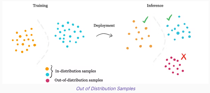
- Out-of-distribution (OOD)
Out-of-distribution (OOD) data refers to data that is different from the data used to train the machine learning model. For example, data collected in a different way, at a different time, under different conditions, or for a different task than the data on which the model was originally trained. An illustration is shown below:
- Overfitting
Overfitting occurs when the machine learning model cannot generalize. The model begins to predict heavily towards the distribution of the developmental dataset which can hurt the model’s predictions on the operational dataset. Overfitting happens due to several reasons, such as:
The training data size is too small and does not contain enough data samples to accurately represent all possible input data values.
The training data contains large amounts of irrelevant information, called noisy data.
The model trains for too long on a single sample set of data.
The model complexity is high, so it learns the noise within the training data.
P
- P-Value
A p-value, or probability value, is a number describing how likely it is that your data would have occurred under the null hypothesis of your statistical test.
- Parity
Parity, in data analysis, measures the statistical independence between class labels and metadata factors using a Chi-Square Test of Independence. A lack of independence indicates bias. See bias.
- Perception-based Hash
Hashing algorithms designed to remain unchanged on very similar inputs. They are designed to detect similar characteristics such as images that have only changed in color, brightness or compression method. So-called pHashes, allow for the comparison of two images by looking at the number of different bits between the input and a second image. This difference is known as the Hamming Distance.
See Hamming Distance
- Pooling Layer
Layers within a convolutional neural network, also known as downsampling layers. Similar to the convolutinal layer, they typically sweep across the output of a convolutional layer and apply aggregation functions using a similar kernel calculation to the output. A lot of information is lost in the pooling layer but they reduce complexity, improve efficiency and limit the risk of overfitting to the developmental dataset. The functions include minimul pooling, maximum pooling and average pooling.
- Precision
A measure of how often a machine learning model correctly predicts the positive class. It is defined as the True Positive Rate (TP) rate divided by the sum of the True Positive Rate (TP) and False Positive Rate (FP) rates.
\(Precision = \frac{TP}{( TP + FP )}\)
where:
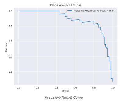
- Precision Recall Curve
A plot which shows precision (Y Axis) vs. recall (X axis) scores for one or more machine learning models as a function of the confidence level to make a prediction. In general, as confidence levels drop, precision decreases as recall increases. The curves are used to visualize the accuracy of a model using various measures including F1-score, Area Under the Curve (AUROC) and Average Precision (AP). An example is shown below:
- Principal Component Analysis (PCA)
Principal component analysis (PCA) is a linear dimensionality reduction technique with applications in exploratory data analysis, visualization and data preprocessing. The data is linearly transformed onto a new coordinate system such that the directions (principal components) capturing the largest variation in the data can be easily identified.
- Probability Distribution
A Probability Distribution is a mathematical function that gives the probabilities of occurrence of different possible random outcomes for an experiment. It can be defined for both discrete and continuous variables.
Q
R
- Recall
A measure of the accuracy of a machine learning model. It is the ability of a model to find all of the relevant cases within a data set. It is defined as the True Positive Rate (TP) over the sum of the True Positive Rate and False Negative Rate (FN).
\(Recall = \frac{TP}{( TP + FN)}\)
where:
- Receiver Operating Characteristic (ROC) Curve
A curve frequently used to evaluate the performance of binary classification algorithms. It provides a graphical representation of a classifier’s performance. It plots the true positive rate vs the false positive rate at a variety of thresholds. An example image is shown below:
- Regularized Autoencoder
A type of autoencoder used mostly in classification tasks. Types include Sparse, Denoising and Contractive. Regularization is a method for constraining the model in order to prevent overfitting and improve its ability to generalize to new data.
- Riemannian Manifold
A manifold where distances and angles can be measured. Type of manifold where divergence can be measured.
- ROC Curve
S
- Sparse Autoencoder (SAE)
A type of autoencoder inspired by the sparse coding hypothesis in neuroscience with the idea that more relevant information will be encoded in a machine learning network if fewer nodes are activated during any single input. By penalizing activation of multiple nodes, it is hoped that more relevant information is encoded rather than passing redundant information.
- Statistical Independence
Two events are statistically independent of one another if the probability of one or either event occurring is not affected by the occurrence or nonoccurrence of the other event.
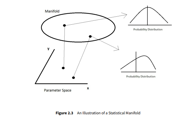
- Statistical Manifold
An abstract space where each point is a probability distribution. An illustration of the conceptis shown below:
- Statistics
Statistics is a branch of applied mathematics that involves the collection, description, analysis, and inference of conclusions from quantitative data.
- Sufficiency
Sufficiency, in the context of data analysis and the DataEval tool, is the notion that the model and/or dataset are capable of satisfying the operational requirements.
See Bayes Error Rate (BER) and Upper-bound Average Precision (UAP).
- Supervised Learning
Supervised Learning is a category of machine learning that uses labeled datasets to train algorithms to predict outcomes and recognize patterns. Unlike unsupervised learning, supervised learning algorithms are given labeled training data to learn the relationship between the inputs and the outputs.
T
- TensorFlow
TensorFlow is a free and open-source software library for machine learning and artificial intelligence. It can be used across a range of tasks but focuses on training and inference of Deep Neural Networks (DNNs)`.
- Torch (PyTorch)
Torch (or Pytorch) is an open-source machine learning library. One of its core packages provides a flexible N-dimensional array (also called a Tensor) data structure used by many machine learning algorithms. It supports routines for manipulation and calculation using Tensors. PyTorch is a library written for the Python programming language.
- True Negative Rate (TN)
A measure of machine learning model accuracy. It measures the frequency a negative prediction was found for a negative ground truth value.
See Confusion Matrix
- True Positive Rate (TP)
A measure of machine learning model accuracy. It measures the frequency a positive prediction was found for a positive ground truth value.
See Confusion Matrix
U
- Unsupervised Learning
Unsupervised learning is a branch of machine learning that learns from data without human supervision. Unlike Supervised Learning, unsupervised machine learning models are given unlabeled data and allowed to discover patterns and insights without any explicit guidance or instruction.
- Upper-bound Average Precision (UAP)
Object detection equivalent of Bayes Error Rate. An estimate of an upper bound on performance for an object detection model on a dataset.
V
- Variance
In probability theory and statistics, variance is the expected value of the squared deviation from the mean of a random variable. Variance is a measure of dispersion from the average value.
- Variational Autoencoder: (VAE)
A type of autoencoder used extensively in generative models (for example Large Language Models (LLMs)) because of its ability to generate new content. The encoder maps each data point (such as an image) from a large complex dataset into a distribution (for example Gaussian) within a latent space or encoded space, rather than a single point.