How to add intrinsic factors to Metadata
Problem Statement
When performing analysis on datasets, metadata may sometimes be sparse or unavailable. Adding metadata to a dataset for analysis may be necessary at times, and can come in the forms of calculated intrinsic values or additional information originally unavailable on the source dataset.
This guide will show you how to add in the calculated statistics from DataEval’s
imagestats() function to the metadata for bias analysis.
When to use
Adding metadata factors should be done when little or no metadata is available on the dataset, or to gain insights specific to metadata of interest that is not present natively in the dataset metadata.
What you will need
A dataset to analyze
A Python environment with the following packages installed:
dataeval[all]
Getting Started
First import the required libraries needed to set up the example.
from maite_datasets.image_classification import CIFAR10

from dataeval.data import Metadata, Select
from dataeval.data.selections import Limit, Shuffle
from dataeval.metrics.bias import balance, diversity, parity
from dataeval.metrics.stats import imagestats
Load the dataset
Begin by loading in the CIFAR-10 dataset.
The CIFAR-10 dataset contains 60,000 images - 50,000 in the train set and 10,000 in the test set. We will use a shuffled sample of 20,000 images from both sets.
# Load in the CIFAR10 dataset and limit to 20,000 images with random shuffling
cifar10 = Select(CIFAR10("data", image_set="base", download=True), [Limit(20000), Shuffle(seed=0)])
print(cifar10)
Select Dataset
--------------
    Selections: [Limit(size=20000), Shuffle(seed=0)]
    Selected Size: 20000

CIFAR10 Dataset
---------------
    Transforms: []
    Image_set: base
    Metadata: {'id': 'CIFAR10_base', 'index2label': {0: 'airplane', 1: 'automobile', 2: 'bird', 3: 'cat', 4: 'deer', 5: 'dog', 6: 'frog', 7: 'horse', 8: 'ship', 9: 'truck'}, 'split': 'base'}
    Path: /dataeval/docs/source/notebooks/data/cifar10
    Size: 60000
Inspect the metadata
You can begin by inspecting the available factor names in the dataset.
metadata = Metadata(cifar10)
print(f"Factor names: {metadata.factor_names}")
Factor names: ['id', 'batch_num']
A quick check of the balance() of the single factor will show no mutual information
between the classes and the batch_num which indicates the on-disk binary file the image
was extracted from.
# Balance at index 0 is always class
balance(metadata).balance[1]
np.float64(0.00040600440845854006)
Add image statistics to the metadata
In order to perform additional bias analysis on the dataset when no meaningful metadata
are provided, you will augment the metadata with statistics of the images using the
imagestats() function.
Begin by running imagestats on the dataset and adding the factors to the metadata.
# Calculate image statistics
stats = imagestats(cifar10)

# Append the factors to the metadata
metadata.add_factors(stats.factors())
Note
When calculating imagestats() for an object detection dataset, you will want
to provide per_box=True to get statistics calculated for each target.
Next you will add the imagestats output to the metadata as factors, and exclude
factors that are uniform or without significance.
Additionally, you will specify a binning strategy for continuous statistical factors, which are, for our purposes, continuous. For this example, bin everything into 10 uniform-width bins.
# Exclude dimension statistics (as CIFAR10 images are all of uniform shape) and the batch_num
metadata.exclude = [
    "aspect_ratio",
    "width",
    "height",
    "depth",
    "channels",
    "size",
    "missing",
    "batch_num",
    "offset_x",
    "offset_y",
    "distance_center",
    "distance_edge",
]

# Provide binning for the continuous statistical factors using 10 uniform-width bins for each factor
keys = ("mean", "std", "var", "skew", "kurtosis", "entropy", "brightness", "darkness", "sharpness", "contrast", "zeros")
metadata.continuous_factor_bins = dict.fromkeys(keys, 10)
Perform bias analysis
Now you can run the bias analysis functions balance(), diversity() and
parity() on the dataset metadata augmented with intrinsic statistical factors.
balance_output = balance(metadata)
_ = balance_output.plot()
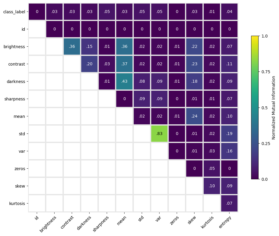
Notice the very high mutual information between the variance and standard deviation of image intensities, which is expected. Mean image intensity correlates with brightness, darkness, and contrast. However, none of the intrinsic factors correlate strongly with class label.
_ = balance_output.plot(plot_classwise=True)
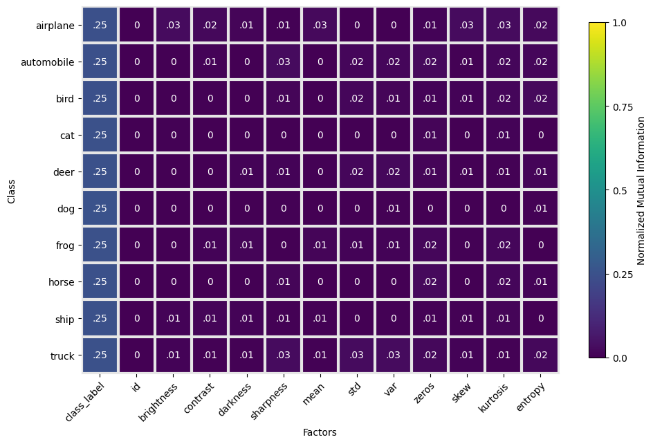
Classwise balance also indicates minimal correlation of image statistics and individual classes. Uniform mutual information between individual classes and all class labels indicates balanced class representation in the subsampled dataset.
diversity_output = diversity(metadata)
_ = diversity_output.plot()
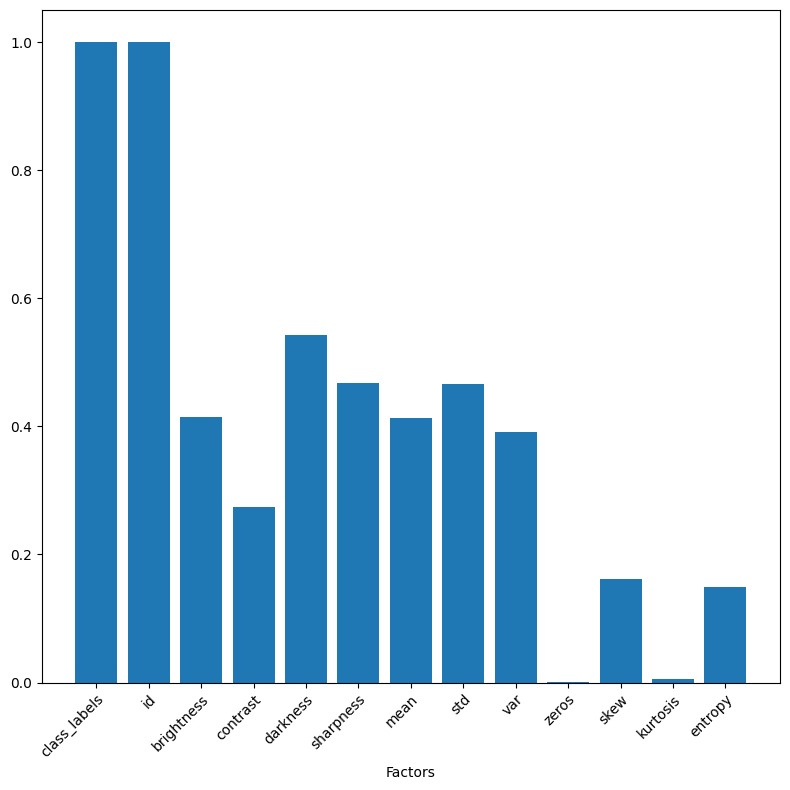
The diversity index also indicates uniform sampling of classes within the dataset. The apparently low diversity of kurtosis across the dataset may indicate an inadequate binning strategy (for metric computation) given that the other statistical moments appear to be more evenly distributed. Further investigation and iteration could be done to assess sensitivity to binning strategy.
parity_output = parity(metadata)
parity_output.to_dataframe()
/dataeval/src/dataeval/metrics/bias/_parity.py:147: UserWarning: Factors ['id', 'brightness', 'contrast', 'darkness', 'sharpness', 'mean', 'std', 'var', 'zeros', 'skew', 'kurtosis', 'entropy'] did not meet the recommended 5 occurrences for each value-label combination.
  warnings.warn(
| score | p-value | |
|---|---|---|
| id | 180000.00 | 0.49 |
| brightness | 2823.68 | 0.00 |
| contrast | 2164.86 | 0.00 |
| darkness | 2553.80 | 0.00 |
| sharpness | 4037.49 | 0.00 |
| mean | 2676.55 | 0.00 |
| std | 3777.54 | 0.00 |
| var | 3623.48 | 0.00 |
| zeros | 105.84 | 0.01 |
| skew | 1921.95 | 0.00 |
| kurtosis | 541.97 | 0.00 |
| entropy | 2811.58 | 0.00 |
You can now augment your datasets with additional metadata information, either from
additional sources or using dataeval statistical functions for insights into your data.