How to detect undersampled data subsets
Problem Statement
For most computer vision tasks like image classification and object detection, we often have a lot of images, but certain subsets of the images can be undersampled, such as label, style within a label, etc. A way to detect this regional sparsity is through coverage analysis.
To help with this, DataEval has introduced a coverage() function, that provides a user with example images which have few similar instances within the provided dataset.
When to use
The coverage function should be used when you have lots of images, but only a small fraction from certain regimes/labels.
What you will need
Image classification dataset.
Autoencoder trained on image classification dataset for dimension reduction (e.g. through the
AETrainerclass).A Python environment with the following packages installed:
dataevalordataeval[all]tabulate
Setting up
Let’s import the required libraries needed to set up a minimal working example
import matplotlib.pyplot as plt
import numpy as np
import torch
import torch.nn as nn
from maite_datasets.image_classification import MNIST
from sklearn.manifold import TSNE

from dataeval.data import Embeddings, Metadata, Select
from dataeval.data.selections import Limit
from dataeval.metrics.bias import coverage
Load the data
Load the MNIST data and create the training dataset.
# Set seeds
torch.manual_seed(14)

transforms = [
    lambda x: x / 255.0,  # scale to [0, 1]
    lambda x: (x - 0.1307) / 0.3081,  # normalize
    lambda x: x.astype(np.float32),  # convert to float32
]

# MNIST with mean 0 unit variance
train_ds = MNIST(root="./data", image_set="train", transforms=transforms, download=True)

# Select a subset of the dataset
subset = Select(train_ds, Limit(2000))
In this tutorial, we will use an autoencoder to reduce the dimension of the MNIST images.
# Define model architecture
class Autoencoder(nn.Module):
    def __init__(self):
        super().__init__()
        self.encoder = nn.Sequential(
            # 28 x 28
            nn.Conv2d(1, 4, kernel_size=5),
            # 4 x 24 x 24
            nn.ReLU(True),
            nn.Conv2d(4, 8, kernel_size=5),
            nn.ReLU(True),
            # 8 x 20 x 20 = 3200
            nn.Flatten(),
            nn.Linear(3200, 10),
            # 10
            nn.Sigmoid(),
        )
        self.decoder = nn.Sequential(
            # 10
            nn.Linear(10, 400),
            # 400
            nn.ReLU(True),
            nn.Linear(400, 4000),
            # 4000
            nn.ReLU(True),
            nn.Unflatten(1, (10, 20, 20)),
            # 10 x 20 x 20
            nn.ConvTranspose2d(10, 10, kernel_size=5),
            # 24 x 24
            nn.ConvTranspose2d(10, 1, kernel_size=5),
            # 28 x 28
            nn.Sigmoid(),
        )

    def forward(self, x):
        x = self.encoder(x)
        x = self.decoder(x)
        return x

    def encode(self, x):
        x = self.encoder(x)
        return x
For computational reasons, we will simply load the trained autoencoder. See the how-to How to create image embeddings with an autoencoder for more information on how to train an autoencoder.
# The trained autoencoder was trained for 1000 epochs
sd = torch.load("models/ae", weights_only=True)
model = Autoencoder()
model.load_state_dict(sd)
<All keys matched successfully>
For the purposes of this example, we will take only the first 2000 entries of the data.
# Calculate the embeddings and extract the labels from the dataset
embeddings = Embeddings(subset, batch_size=64, model=model).to_tensor()
labels = Metadata(subset).class_labels
To visualize the encodings, we will use TSNE on them to view separation.
# Visualize 10d as 2d with TSNE
tsne = TSNE(n_components=2)
red_dim = tsne.fit_transform(embeddings.cpu().numpy())
# Plot results with color being label
fig, ax = plt.subplots()
scatter = ax.scatter(
    x=red_dim[:, 0],
    y=red_dim[:, 1],
    c=labels,
    label=labels,
)
ax.legend(*scatter.legend_elements(), loc="upper right", ncols=2)
plt.show()
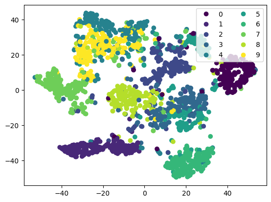
Some good separation, but you can see a few images in the “gaps”. This could be an artifact of dimension reduction, or suggest that we have poor coverage for some covariates.
# Use data adaptive cutoff
cvrg = coverage(embeddings, radius_type="adaptive")
# Plot the least covered 1%
f, axs = plt.subplots(4, 5, figsize=(5, 5))
axs = axs.flatten()
for count, i in enumerate(axs):
    idx = cvrg.uncovered_indices[count]
    i.imshow(np.squeeze(train_ds[idx][0]), cmap="gray")
    i.set_axis_off()
    i.title.set_text(int(labels[idx]))
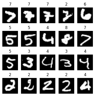
The Coverage tool identified that in this set of 2000 images, there is potential under-coverage when it comes to wonky 2s and 7s. Other digits have some undercovered instances, but could be they are just outliers.