Assess an unlabeled data space¶

This guide provides a beginner friendly introduction to exploratory data analysis when labels are not available.

Estimated time to complete: 10 minutes

Relevant ML stages: Data Engineering

Relevant personas: Data Engineer, Data Scientist

What you’ll do¶

• Construct embeddings by inferencing the PASCAL VOC 2012 through a model

• Analyze clustered embeddings to find outliers

• Run additional analysis to find gaps in data coverage

What you’ll learn¶

• Learn to use cluster based algorithms to measure dataset quality without labels

• Learn to distinguish if an image is an outlier or is underrepresented

• Learn to determine if flagged images should be added or removed

What you’ll need¶

• Basic familiarity with Python

Background¶

Before building predictive models, it’s essential to identify outliers and ensure that data groups accurately reflect the underlying distribution. When labels are unavailable do to things like unsupervised learning, initial data curration, or expensive annotations, analysis can still be done on the images alone. We do this by considering images to be geometric points in a high-dimensional abstract space called feature space. By understanding how the data examples are distributed in feature space, you will become able to make the assessments you need. Specifically by grouping data points (i.e. images) into clusters, you can explore the natural structure of the dataset to reveal hidden patterns and potential anomalies. Measuring coverage goes a step further by quantifying how well the clusters represent the entire dataset to ensure that no significant portion of the feature space is being overlooked.

These techniques are critical for evaluating the quality and representativeness of your data, helping to avoid biases and missing information or overfitting issues in your models. By understanding the space your data occupies and how it groups, you can build more robust and reliable models that generalize well in real-world applications.

Setup¶

You’ll begin by importing the necessary libraries for this tutorial.

import torch

# Dataset
from maite_datasets.object_detection import VOCDetectionTorch

# Data structures
from dataeval.data import Embeddings, Images

# Coverage
from dataeval.metrics.bias import coverage

# Clustering
from dataeval.metrics.estimators import clusterer

# Model
from dataeval.utils.torch.models import ResNet18

# Set default torch device for notebook
device = torch.device("cuda" if torch.cuda.is_available() else "cpu")
torch.set_default_device(device)

Constructing Embeddings¶

An important concept in many aspects of machine learning is Dimensionality Reduction. While this step is not always necessary, it is good practice to use embeddings over raw images to improve the speed and memory efficiency of many workflows without sacrificing downstream performance.

In this section, you will use a pretrained ResNet18 model to reduce the dimensionality of the VOC dataset.

Define model architecture¶

In the cell below, you will instantiate a wrapper class for the ResNet18 model that automatically sets common parameters. Since the model has many layers, visit the ResNet18 reference page for more information on its architecture.

resnet = ResNet18()

# Uncomment the line below to see the model architecture in detail
# print(resnet)

Downloading: "https://download.pytorch.org/models/resnet18-f37072fd.pth" to /home/dataeval/.cache/torch/hub/checkpoints/resnet18-f37072fd.pth

Download VOC dataset¶

Now you will download the train split using the VOCDetection class. The train split contains 5717 images with a varying number of targets in each image. This makes it useful for determining gaps in coverage.

To run this tutorial with your own dataset, swap dataset with a torch.utils.data.Dataset subclass and remove the print(dataset.info()) call below.

# Load the training dataset
dataset = VOCDetectionTorch(root="./data", year="2012", image_set="train", download=True)

print(dataset)

dataset[0][0].shape

VOCDetectionTorch Dataset
-------------------------
    Year: 2012
    Transforms: []
    Image_set: train
    Metadata: {'id': 'VOCDetectionTorch_train', 'index2label': {0: 'aeroplane', 1: 'bicycle', 2: 'bird', 3: 'boat', 4: 'bottle', 5: 'bus', 6: 'car', 7: 'cat', 8: 'chair', 9: 'cow', 10: 'diningtable', 11: 'dog', 12: 'horse', 13: 'motorbike', 14: 'person', 15: 'pottedplant', 16: 'sheep', 17: 'sofa', 18: 'train', 19: 'tvmonitor'}, 'split': 'train'}
    Path: /dataeval/docs/source/notebooks/data/vocdataset/VOCdevkit/VOC2012
    Size: 5717

torch.Size([3, 442, 500])

It is good to notice a few points about each dataset:

• Number of datapoints

• Image size

These two values give an estimate of the memory impact that the dataset has. The following step will modify the resize size by creating model embeddings for each image to reduce this impact.

Extract embeddings¶

Now it is time to process the datasets through your model. Aggregating the model outputs gives you the embeddings of the data. This will be helpful in determining clusters that are representative of your dataset

The batch_voc() function is specifically designed to handle specific behaviors when using a PyTorch Dataloader on the VOC dataset.

# Extract embeddings from the dataset using the ResNet18 model after applying transforms
embeddings = Embeddings(
    dataset=dataset,
    batch_size=64,
    model=resnet,
    transforms=resnet.transforms(),
).to_tensor()

embeddings.shape

torch.Size([5717, 128])

The shape has been reduced to (128,). This will greatly improve the performance of the upcoming algorithms without impacting the accuracy of the results. Notice that the original number of images, 5717, is the same as before you created image embeddings.

Embeddings create a more performant representation of the data than simply resizing but are more computational expensive. In most cases, this step is not the bottleneck of a pipeline and is generally considered worth the improvement in performance of downstream tasks.

Cluster the Embeddings¶

In this section, you will use the embeddings you generated to create clusters. A cluster is a group of images that have similar characteristics. Based on this information, images can be found that are either too similar or too dissimilar. Both cases can lead to performance degradation of downstream tasks such as data analysis or model training.

Normalize embeddings¶

Before clustering can be done, the embeddings need to be normalized between 0 and 1 for the clusterer() to properly group them. Let’s look at the current spread of the embeddings values.

print(f"Max value: {embeddings.max()}")
print(f"Min value: {embeddings.min()}")

Max value: 3.533177375793457
Min value: -4.198641300201416

These are certainly not between 0 and 1 but the next step will fix that by doing min-max normalization.

# Puts the embeddings onto the unit interval [0-1]
normalized_embs = (embeddings - embeddings.min()) / (embeddings.max() - embeddings.min())

print(f"Max value: {normalized_embs.max()}")
print(f"Min value: {normalized_embs.min()}")

Max value: 1.0
Min value: 0.0

Now your embeddings are between 0 and 1!

Create clusters¶

The data is now ready to be clustered. Run the normalized embeddings through the clusterer() function to generate the ClustererOutput class.

output = clusterer(normalized_embs)

You have successfully clustered your image embeddings! The ClustererOutput contains several attributes related to clusters such as the minimum spanning tree and linkage array. For this tutorial, you can focus on the ClustererOutput.find_outliers() method to analyze the quality of the dataset. For additional use cases, additional benefits, and even alternative methods, read more about clustering in DataEval’s documentation.

Visualize the outputs¶

While generating the clusters, individual samples were flagged by the clusterer() for potentially being outliers or duplicates. In this section, you will look at the flagged images and decide on corrective measures to improve the quality of the data.

Let’s take a quick look at the categories of flagged images:

• duplicates

• outliers

Let’s take a look at each of these in turn.

Duplicates¶

When evaluating the clusters, if two or more data points are within a certain distances from each other, the index of each data point will be marked as a duplicate.

To access the duplicates, the ClustererOutput.find_duplicates() function will return a list of indices it has flagged.

For this tutorial, we will not focus on duplicates as no images are flagged in the PASCAL 2012 VOC dataset.

Outliers¶

Outliers are individual data points that did not fit within the radius of any cluster. Potential outliers are outliers who fall within a small distance from the radius and may become part of the cluster if more data is acquired.

It is important to identify outliers as they can skew the training distribution away from the operational distribution, which can lead to performance degradation.

Let’s see how many images were flagged by calling ClustererOutput.find_outliers().

outliers = output.find_outliers()

print(f"Number of outliers: {len(outliers)}")

Number of outliers: 3279

That is a significant number of outliers. A quick calculation of the percent of outliers in the dataset can be done.

print(f"Percent of outliers: {(100 * len(outliers) / len(dataset)):.2f}%")

Percent of outliers: 57.36%

It is always a good idea to view a few of these images to get a better understand of why they were flagged.

Plot some samples¶

You are free to choose which set of images you would like to examine. Take a moment to swap out the different indices when calling the plot function by uncommenting your preferred indices calculation. You can also adjust the count parameter if you would like to see more examples.

# To use the flagged outliers, uncomment the line below
indices = outliers

# To use unflagged images, uncomment the line below
# indices = list(set(range(len(dataset))) - set(outliers)

Now run your chosen set of indices through the plot function.

# Use the Images class to access and plot images
images = Images(dataset)

# Plot 6 images from the dataset
_ = images.plot(indices.tolist()[:6], figsize=(12, 8), images_per_row=3)

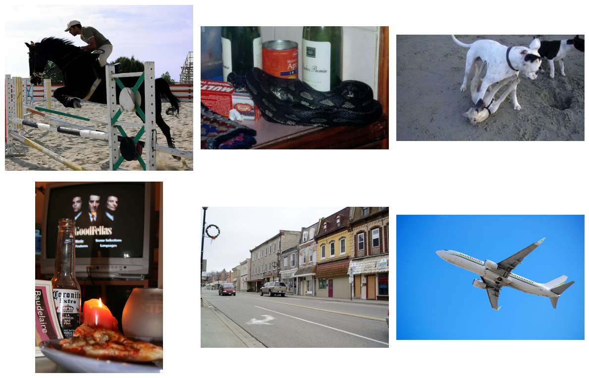
Analyze the flagged images¶

Visualization is a great way to catch initial differences between images in a dataset. However, it is only a preliminary step into identifying the root cause of an outlier. Several initial questions can be asked to ensure outliers are handled properly and represent the underlying distribution of the data.

Initial questions¶

When looking at the above samples, here is a shortlist of questions you should use to determine the appropriate data cleaning step:

1. Are there unexpected artifacts in the image?

   • Examples: Data collection, processing, and visualization can cause discoloration, blurriness, etc

   • Solution: Ensure images are normalized with the right values, channel order is correct, color scheme is consistent

   • See our in-depth Data Cleaning tutorial to explore these types of outliers

2. Do you have enough data?

   • Examples: Less data points in each cluster can lead to higher deviation and more outliers

   • Solution: Adding more data can help make the clusters more robust to the variations in images

3. Do the images provide useful information?

   • Examples: Image attributes like number of duplicates, pixel intensity, etc can cause the clusterer to become biased to the wrong information

   • Solution: Determine if the data represents the whole operational distribution

   • This solution will be explored in the following section

This is only a shortlist of potential causes for outliers based on pixel values. Over time you will add more questions and solutions that suit your specific needs.

Outliers and edge cases¶

The most common way to clean data is to remove the outliers entirely. This provides an easy and efficient way to stabilize the training distribution. However, this can lead to shortages of data, class imbalances, and a loss of potentially useful information. It is also important to remember that outliers and edge cases are different. Edge cases are statistically rare events that are relevant to the downstream task. This is why it is important to carefully look at outliers to ensure they are irrelevant.

One way to determine if an image is relevant even when the total distribution considers it an outlier is to measure its coverage.

Measure image coverage¶

Coverage is the measurement of the representation of an image’s variations in a feature’s space. When an image does not have enough variations, it is underrepresented. In this section, you will test for any gaps in the coverage of the dataset to find underrepresented images.

Calculate coverage¶

The coverage() function will return a list of image indices that it finds to be underrepresented. This means it does not have enough similar images around it. This should sound familiar as outliers have a very similar situation. However, underrepresented images should be handled different than outliers. More on this in the next section.

cov = coverage(embeddings=normalized_embs)

print(f"Number of uncovered images: {len(cov.uncovered_indices)}")

Number of uncovered images: 57

You can plot a few images using the same function as before.

_ = cov.plot(images=images, top_k=3)

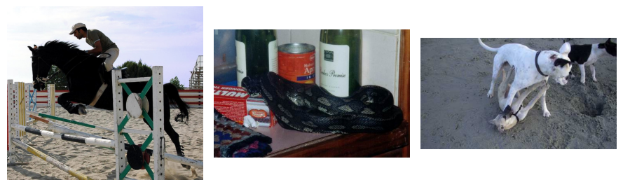
Now you have seen a few examples of images that were flagged as uncovered. You will compare this information with the outliers found earlier to determine which actions should be taken.

uncovered_outliers = set(cov.uncovered_indices.tolist()).intersection(set(outliers))

print(f"Number of outliers found as uncovered images: {len(uncovered_outliers)}")

Number of outliers found as uncovered images: 57

Handling flagged images¶

You now have enough information to determine what should be done with these images. If they are both flagged as outliers and underrepresented, handle them first as missing coverage and then as outliers if solutions cannot be acted on.

Missing coverage¶

For the images with a gap in coverage, the characteristics of the individual images need additional samples. This can be done by collecting more images of similar information (pose, scene, color, labels if available) or through additional augmentations.

Outliers¶

Outliers can be handled by additional sampling but typically are removed as they either do not contain enough relevant information or would cause a shift in the underlying distribution if similar items were added.

Conclusion¶

In this tutorial you have learned to create image embeddings for more efficient calculations, to use cluster based algorithms to find outliers, to check for gaps in coverage, and to make decisions on possible solutions.

Good luck with your data!

What’s next¶

In addition to exploring a dataset in its feature space, DataEval offers additional tutorials on exploratory data analysis:

• Clean a dataset with the labels in the Data Cleaning Guide

• Identify Bias and Correlations in your metadata

Explore deeper explanations on topics such as clustering, coverage, and outliers in the Concept pages.

On your own¶

Once you are familiar with DataEval and data analysis, run this analysis on your own dataset. When you do, make sure that you analyze all of your data and not just the training set.