How to detect uncertainty drift with a MAITE model
Problem statement
When a model is deployed, the model itself is a sensitive instrument for distribution shift: as operational data moves into regions the model was not trained on, its predictions grow less confident. The Shannon entropy of the predicted class probabilities summarizes that confidence — low entropy is a peaked, confident prediction; high entropy means the model is hedging. If the distribution of per-prediction entropy shifts upward, the model is increasingly operating in its uncertainty regions: a strong, label-free drift signal. See the uncertainty-based drift detection concept page for the theory and trade-offs.
To turn predictions into an uncertainty feature, DataEval needs to decode the model’s raw output into a
(n_predictions, n_classes) array of class scores. The drift-with-uncertainty
tutorial does this by wrapping a model in TorchExtractor with a
hand-written postprocess_fn specific to that model’s output format.
This guide shows the alternative for models that conform to DataEval’s opinionated ONNX/LiteRT contract: a
OnnxImageClassifier (a MAITE image_classification.Model) paired with ScoresExtractor
decodes the predictions for you — no postprocess_fn required — and feeds straight into UncertaintyExtractor
and a drift detector.
When to use
Use the OnnxImageClassifier + ScoresExtractor path when you want to:
Monitor a deployed ONNX or LiteRT model for distribution shift without operational ground-truth labels
Reuse a model that already ships with a
model-metadata.jsondescribing its input/output contractAvoid writing and maintaining a model-specific
postprocess_fnto decode raw predictions
The same pattern works for object detection with OnnxObjectDetector; ScoresExtractor flattens
per-detection scores so the rest of the workflow is identical.
What you will need
An ONNX (or LiteRT) model that conforms to the opinionated contract, plus its
model-metadata.json. In production you bring your own; in the Build a model section below you export a small one so this guide is self-contained.A reference dataset (in-distribution) and an operational stream to monitor. This guide uses
MNISTas in-distribution andCIFAR-10as the shifted stream.A Python environment with the following packages installed:
dataeval[onnx]maite-datasetstorch(only to export the demo model)
Getting started
Import the libraries needed for a minimal working example.
import json
import warnings
from pathlib import Path

import matplotlib.pyplot as plt
import numpy as np
import torch
from maite_datasets.image_classification import CIFAR10, MNIST
from torch import nn

from dataeval.config import set_seed
from dataeval.data import Indices, Limit, Select, Shuffle
from dataeval.extractors import ScoresExtractor, UncertaintyExtractor
from dataeval.models import OnnxImageClassifier
from dataeval.shift import DriftWasserstein

set_seed(0, all_generators=True)
Build a conforming model for the demo
OnnxImageClassifier wraps two artifacts you would normally already have for a deployed model:
the model file (
.onnxor.tfliteforLiteRtImageClassifier), anda
model-metadata.jsondeclaring the input/output contract — task, input channels and size, and the number of classes the model scores.
Because this guide is self-contained, you quickly train a small MNIST classifier and export it. This block is demo
scaffolding — in your own workflow you would skip it and point OnnxImageClassifier at the model and
metadata you already have.
The exported model emits a softmax scores output (probabilities), which is exactly what the opinionated
classification contract expects.
class TinyCNN(nn.Module):
    """A small MNIST classifier emitting raw logits."""

    def __init__(self) -> None:
        super().__init__()
        self.net = nn.Sequential(
            nn.Conv2d(1, 16, 3, padding=1),
            nn.ReLU(),
            nn.MaxPool2d(2),
            nn.Conv2d(16, 32, 3, padding=1),
            nn.ReLU(),
            nn.MaxPool2d(2),
            nn.Flatten(),
            nn.Linear(32 * 7 * 7, 10),
        )

    def forward(self, x: torch.Tensor) -> torch.Tensor:
        return self.net(x)


class WithSoftmax(nn.Module):
    """Wrap a logits model so its ONNX ``scores`` output is a probability distribution."""

    def __init__(self, base: nn.Module) -> None:
        super().__init__()
        self.base = base

    def forward(self, x: torch.Tensor) -> torch.Tensor:
        return torch.softmax(self.base(x), dim=1)
# Train the demo classifier on a small slice of MNIST (a few seconds on CPU).
mnist_train = MNIST("./data", image_set="train", download=True)
train_ids = np.random.default_rng(0).permutation(len(mnist_train))[:4000]
x_train = torch.tensor(np.stack([np.asarray(mnist_train[i][0], dtype=np.float32) / 255.0 for i in train_ids]))
y_train = torch.tensor(np.stack([np.asarray(mnist_train[i][1]).argmax() for i in train_ids]))

model = TinyCNN()
optimizer = torch.optim.Adam(model.parameters(), lr=1e-3)
loss_fn = nn.CrossEntropyLoss()
model.train()
for _ in range(3):
    order = torch.randperm(len(x_train))
    for start in range(0, len(x_train), 128):
        batch = order[start : start + 128]
        optimizer.zero_grad()
        loss_fn(model(x_train[batch]), y_train[batch]).backward()
        optimizer.step()
model.eval()
TinyCNN(
  (net): Sequential(
    (0): Conv2d(1, 16, kernel_size=(3, 3), stride=(1, 1), padding=(1, 1))
    (1): ReLU()
    (2): MaxPool2d(kernel_size=2, stride=2, padding=0, dilation=1, ceil_mode=False)
    (3): Conv2d(16, 32, kernel_size=(3, 3), stride=(1, 1), padding=(1, 1))
    (4): ReLU()
    (5): MaxPool2d(kernel_size=2, stride=2, padding=0, dilation=1, ceil_mode=False)
    (6): Flatten(start_dim=1, end_dim=-1)
    (7): Linear(in_features=1568, out_features=10, bias=True)
  )
)
Export the trained model to ONNX and write the matching model-metadata.json. The metadata declares a single-channel
(GRAYSCALE) 28x28 input and 10 output classes — the contract OnnxImageClassifier reads to build model
input and validate output.
Path("data").mkdir(exist_ok=True)
model_path = "data/mnist-demo.onnx"
metadata_path = "data/mnist-demo-metadata.json"

with warnings.catch_warnings():
    warnings.simplefilter("ignore")
    torch.onnx.export(
        WithSoftmax(model).eval(),
        (torch.zeros(1, 1, 28, 28),),
        model_path,
        input_names=["image"],
        output_names=["scores"],
        dynamic_axes={"image": {0: "batch"}, "scores": {0: "batch"}},
        opset_version=13,
        dynamo=False,
    )

_ = Path(metadata_path).write_text(
    json.dumps({
        "interface": {"name": "JATIC_ONNX", "version": "v1"},
        "io": {
            "batchSize": -1,
            "interface": "IMAGE_CLASSIFICATION",
            "input": {"channels": "GRAYSCALE", "height": 28, "width": 28},
            "output": {"nClasses": 10},
        },
    }),
    encoding="utf-8",
)
Load the datasets
You need three exchangeable in-distribution slices plus a shifted stream:
train and val — two disjoint, same-distribution slices of MNIST; the train-vs-val distance calibrates the baseline for “normal” variation between in-distribution samples.
test — a third disjoint MNIST slice held out from calibration; because it is exchangeable with train and val, the detector should report no drift here.
cifar — CIFAR-10 imagery, a genuinely shifted operational stream (natural color photos rather than handwritten digits); the detector should report drift here.
The opinionated input builder handles the format differences automatically: CIFAR-10’s RGB 32x32 images are converted to grayscale and resized to the model’s 28x28 input per the metadata contract — no manual preprocessing needed.
SAMPLES_PER_SPLIT = 200

mnist_test = MNIST("./data", image_set="test", download=True)

# Three disjoint, exchangeable MNIST slices: two references that calibrate the baseline
# (train, val) and a held-out set that should NOT drift (test).
perm = np.random.default_rng(1).permutation(len(mnist_test))
train_idx, val_idx, test_idx = np.array_split(perm[: 3 * SAMPLES_PER_SPLIT], 3)
trainset = Select(mnist_test, Indices(train_idx.tolist()))
valset = Select(mnist_test, Indices(val_idx.tolist()))
testset = Select(mnist_test, Indices(test_idx.tolist()))

# Shifted "operational" data: CIFAR-10 natural images
cifarset = Select(CIFAR10("./data", image_set="test", download=True), [Shuffle(0), Limit(SAMPLES_PER_SPLIT)])

print(f"train: {len(trainset)}  val: {len(valset)}  test: {len(testset)}  cifar: {len(cifarset)}")
train: 200 val: 200 test: 200 cifar: 200
Build the uncertainty feature extractor
This is the core of the guide. Three small pieces compose into a single feature extractor:
OnnxImageClassifierloads the model and its metadata and runs inference, returning one(n_classes,)score array per image.ScoresExtractoradapts that MAITEModelinto aFeatureExtractor, stacking per-image scores into an(n_images, n_classes)array.UncertaintyExtractorconverts each row of class probabilities into a single normalized-entropy value.
Note what is absent: there is no postprocess_fn. The opinionated classifier already speaks the
(instances, classes) contract ScoresExtractor expects, so the decoding the tutorial does by hand is handled
for you. Because the model outputs a softmax distribution, use preds_type="probs".
classifier = OnnxImageClassifier(model_path, metadata_path)
scores = ScoresExtractor(classifier)
uncertainty = UncertaintyExtractor(scores, preds_type="probs", normalize=True)

print(uncertainty)
2026-07-02 17:18:06.747394233 [W:onnxruntime:Default, device_discovery.cc:325 DiscoverDevicesForPlatform] GPU device discovery failed: device_discovery.cc:92 ReadFileContents Failed to open file: "/sys/class/drm/card0/device/vendor"
UncertaintyExtractor(scores=ScoresExtractor, preds_type='probs', normalize=True)
Compute uncertainty for each split
Calling the extractor on a dataset returns an (n_images, 1) array of normalized-entropy values — one per image.
h_train = uncertainty(trainset)
h_val = uncertainty(valset)
h_test = uncertainty(testset)
h_cifar = uncertainty(cifarset)

print(
    f"mean entropy -> train: {h_train.mean():.3f}  val: {h_val.mean():.3f}  "
    f"test: {h_test.mean():.3f}  cifar: {h_cifar.mean():.3f}"
)
mean entropy -> train: 0.183 val: 0.190 test: 0.191 cifar: 0.452
Visualize the uncertainty distributions
An empirical CDF (ECDF) makes the shift easy to read: if the CIFAR-10 curve sits to the right of the MNIST curves, the model is systematically more uncertain on the shifted imagery. The in-distribution splits (train, val, test) should overlap closely.
plt.figure()
for label, h in [("train", h_train), ("val", h_val), ("test", h_test), ("cifar", h_cifar)]:
    plt.ecdf(h.flatten(), label=label)
plt.xlabel("Normalized entropy")
plt.ylabel("Cumulative density")
plt.title("Prediction uncertainty by split")
plt.legend()
plt.show()
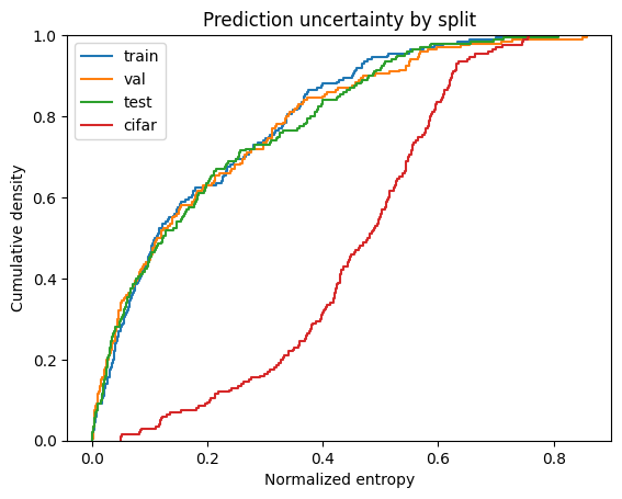
The MNIST splits cluster together while CIFAR-10 is visibly shifted toward higher entropy — exactly what you expect from a classifier encountering data outside its training distribution.
Detect drift with Wasserstein distance
Eyeballing ECDFs is useful, but you want an automated decision. DriftWasserstein measures the
Wasserstein distance between the reference and incoming uncertainty distributions and
flags drift when that distance grows beyond a calibrated baseline.
Unlike most detectors, DriftWasserstein takes two in-distribution references in fit(): a training set and a
validation set. The train-vs-validation distance defines the normal amount of variation between two same-distribution
samples, so the detector only alarms when incoming data is more different from training than validation was.
drift_detector = DriftWasserstein().fit(np.asarray(h_train), np.asarray(h_val))

result_test = drift_detector.predict(np.asarray(h_test))
print(f"MNIST held-out -> drift: {result_test.drifted}  (ratio: {result_test.distance:.2f})")

result_cifar = drift_detector.predict(np.asarray(h_cifar))
print(f"CIFAR-10       -> drift: {result_cifar.drifted}  (ratio: {result_cifar.distance:.2f})")
MNIST held-out -> drift: False  (ratio: 1.07)
CIFAR-10       -> drift: True  (ratio: 18.48)
The held-out MNIST slice stays within the calibrated baseline (no drift), while CIFAR-10 exceeds it (drift detected). The detector turned the visual gap in the ECDF into an automated, label-free alert — and you never had to write a decoder for the model’s output.
On your own
Swap in your own model: drop the demo scaffolding and pass
OnnxImageClassifierthe.onnxandmodel-metadata.jsonyou already ship — orLiteRtImageClassifierfor a.tflitemodel.Swap the operational data: point the shifted split at your real incoming data stream.
Monitor a detector: use
OnnxObjectDetector(orLiteRtObjectDetector) withScoresExtractor— orClasswiseUncertaintyExtractorto break uncertainty down per predicted class.Tune sensitivity: adjust
DriftWasserstein(ratio_threshold=...)to trade off false alarms against missed drift.