Detect drift with prediction uncertainty¶

This guide shows how to monitor a deployed object detector for distribution shift using the model’s own prediction uncertainty as the drift signal.

Estimated time to complete: 10 minutes

Relevant ML stages: Monitoring

Relevant personas: Machine Learning Engineer, T&E Engineer

What you’ll do¶

• Turn a pretrained object detector into a feature extractor with TorchExtractor

• Convert raw detection outputs into per-detection uncertainty with UncertaintyExtractor

• Visualize how the uncertainty distribution differs between in-distribution and shifted data

• Break uncertainty down per predicted class with ClasswiseUncertaintyExtractor

• Detect drift on the uncertainty feature with DriftWasserstein

What you’ll learn¶

• Learn how prediction uncertainty (entropy) can act as a drift feature without ground-truth labels

• Learn how to decode a detection model’s raw output into per-detection class scores with a postprocess_fn

• Learn how a calibrated, validation-anchored detector separates benign variation from genuine drift

What you’ll need¶

• Knowledge of Python

• Beginner knowledge of PyTorch and object detection

• The ultralytics package for the pretrained YOLO detector

Introduction¶

Most drift detectors compare the features of incoming data against a reference set (see the monitoring tutorial). But when you have a deployed model, the model itself is a sensitive instrument: as operational data moves into regions the model was not trained on, its predictions become less confident.

For a classifier — or, here, the classification head of an object detector — confidence can be summarized by the Shannon entropy of the predicted class probabilities. Low entropy means a confident, peaked prediction; high entropy means the model is hedging across classes. If the distribution of per-detection entropy shifts upward on operational data, the model is increasingly operating in its uncertainty regions — a strong, label-free signal that the data has drifted. See the uncertainty-based drift detection concept page for the theory and trade-offs.

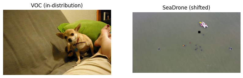
In this tutorial you will use a pretrained YOLOv8 detector and the 2012 VOC dataset as in-distribution data. You will then treat the SeaDrone maritime detection dataset as a shifted operational stream — top-down, drone-captured imagery over open water, a domain the everyday-object detector’s training never covered — and confirm that its prediction uncertainty has drifted while a held-out slice of in-distribution VOC data has not.

Setup¶

You’ll begin by importing the necessary libraries for this tutorial.

import matplotlib.pyplot as plt
import numpy as np
import torch
from maite_datasets.object_detection import SeaDrone, VOCDetection
from torchvision.transforms.functional import resize
from ultralytics import YOLO

from dataeval.config import set_batch_size
from dataeval.data import Indices, Limit, Select, Shuffle
from dataeval.extractors import ClasswiseUncertaintyExtractor, TorchExtractor, UncertaintyExtractor
from dataeval.shift import DriftWasserstein

# Set default torch device for notebook
device = "cuda" if torch.cuda.is_available() else "cpu"

# Set the default batch size used when loading and encoding images
set_batch_size(32)

Creating new Ultralytics Settings v0.0.6 file ✅ 
View Ultralytics Settings with 'yolo settings' or at '/root/.config/Ultralytics/settings.json'
Update Settings with 'yolo settings key=value', i.e. 'yolo settings runs_dir=path/to/dir'. For help see https://docs.ultralytics.com/quickstart/#ultralytics-settings.

More on device and batch size

The device is the piece of hardware where the model and data live in memory; if a GPU is available this notebook uses it, otherwise the CPU. The batch size set above is the default I/O chunk size DataEval uses when streaming images through an extractor. For more on these global settings, see the configuration defaults how-to.

Load the datasets¶

You need two in-distribution references plus a held-out in-distribution set and a shifted set:

• train and val — two disjoint, same-distribution slices of VOC; the train-vs-val distance calibrates the detector’s baseline for “normal” variation between in-distribution samples.

• test — a third disjoint VOC slice, held out from calibration; because it is exchangeable with train and val, the detector should report no drift here.

• drone — SeaDrone maritime imagery, a genuinely shifted operational stream; the detector should report drift here.

To keep the tutorial fast, each split is capped to a small random subset with Select and Limit. Both datasets are already used by other guides, so they are typically cached locally. Raise SAMPLES_PER_SPLIT (or drop the Select wrappers) to run on more data.

SAMPLES_PER_SPLIT = 200

voc = VOCDetection("./data", year="2012", image_set="train", download=True)

# Three disjoint, exchangeable slices of in-distribution VOC data: two references that
# calibrate the baseline (train, val) and a held-out set that should NOT drift (test).
# Drawing all three from the same pool keeps them statistically interchangeable, so the
# train-vs-val baseline genuinely predicts the train-vs-test distance.
perm = np.random.default_rng(0).permutation(len(voc))
train_idx, val_idx, test_idx = np.array_split(perm[: 3 * SAMPLES_PER_SPLIT], 3)
trainset = Select(voc, Indices(train_idx.tolist()))
valset = Select(voc, Indices(val_idx.tolist()))
testset = Select(voc, Indices(test_idx.tolist()))

# Shifted "operational" data: the SeaDrone maritime aerial (drone-captured) detection dataset
droneset = Select(SeaDrone("./data", image_set="val", download=True), [Shuffle(0), Limit(SAMPLES_PER_SPLIT)])

print(f"train: {len(trainset)}  val: {len(valset)}  test: {len(testset)}  drone: {len(droneset)}")

train: 200  val: 200  test: 200  drone: 200

Visualize a sample from each domain¶

Plotting one image from each domain makes the shift concrete: everyday eye-level VOC scenes versus top-down, drone-captured SeaDrone imagery over open water.

fig, (ax_voc, ax_drone) = plt.subplots(1, 2, figsize=(10, 4))
ax_voc.imshow(np.asarray(trainset[0][0]).transpose(1, 2, 0))
ax_voc.set_title("VOC (in-distribution)")
ax_voc.axis("off")
ax_drone.imshow(np.asarray(droneset[0][0]).transpose(1, 2, 0))
ax_drone.set_title("SeaDrone (shifted)")
ax_drone.axis("off")
plt.show()

Build the uncertainty feature extractor¶

DataEval turns any model into a feature extractor via TorchExtractor. To extract uncertainty from a detection model you need two small adapter functions:

• a transforms function that prepares each image for the model (resize to the model’s input size and scale pixel values to [0, 1]), and

• a postprocess_fn that decodes the model’s raw output into a (n_detections, n_classes) array of per-detection class scores.

The postprocess_fn is the bridge between a model’s idiosyncratic output format and the generic (instances, classes) shape that UncertaintyExtractor consumes. The decoder below is specific to YOLOv8’s raw output; a different detector would need its own.

def preprocess_fn(image: torch.Tensor) -> torch.Tensor:
    """Prepare a single image for YOLO: resize to 640x640 and scale to [0, 1]."""
    image = resize(image, size=[640, 640])
    return image.float() / 255.0


def postprocess_fn(output: tuple) -> torch.Tensor:
    """Decode YOLOv8 raw output into per-detection class scores.

    YOLOv8's raw output is a ``(inference_tensor, train_output)`` tuple. We take
    the per-anchor class scores, transpose them to ``(batch, anchors, classes)``,
    and keep only anchors with a meaningful detection (max class probability above
    a small floor), yielding a ``(n_detections, n_classes)`` score tensor.
    """
    _, detections = output
    scores = detections["scores"].cpu().mT  # (B, n_classes, n_anchors) -> (B, n_anchors, n_classes)
    max_probs, _ = torch.sigmoid(scores).max(dim=-1)
    keep = max_probs > 0.05  # drop background/empty anchors
    return scores[keep]

With the adapters defined, load the pretrained detector and wrap it. The TorchExtractor runs the model and returns decoded detection scores; UncertaintyExtractor then converts each detection’s class scores (here logits, since YOLO scores are not normalized) into a single normalized-entropy value.

# Load the underlying torch module from the Ultralytics wrapper
model = YOLO("data/yolov8s.pt").model

# Decode the detector into per-detection class scores
scores = TorchExtractor(
    model,
    transforms=preprocess_fn,
    postprocess_fn=postprocess_fn,
    device=device,
    batch_size=32,
)

# Per-detection normalized entropy: one uncertainty value per detection
uncertainty = UncertaintyExtractor(scores, preds_type="logits", normalize=True)

Why batch_size on the extractor?

TorchExtractor’s batch_size is the model’s forward-pass batch size — how many images go through the network at once — which is distinct from the I/O chunk size Embeddings uses to stream data from disk. Setting it bounds GPU memory during inference regardless of how large each I/O chunk is.

Compute uncertainty for each split¶

Calling the extractor on a dataset returns an (n_detections, 1) array of normalized-entropy values — one per detection across every image in the split.

h_train = uncertainty(trainset)
h_val = uncertainty(valset)
h_test = uncertainty(testset)
h_drone = uncertainty(droneset)

print(f"detections -> train: {len(h_train)}  val: {len(h_val)}  test: {len(h_test)}  drone: {len(h_drone)}")

detections -> train: 14021  val: 11408  test: 11225  drone: 5613

Visualize the uncertainty distributions¶

An empirical CDF (ECDF) makes the shift easy to read: if the SeaDrone curve sits to the right of the VOC curves, the detector is systematically more uncertain on the shifted imagery. The in-distribution splits (train, val, test) should overlap closely.

plt.figure()
for label, H in [("train", h_train), ("val", h_val), ("test", h_test), ("drone", h_drone)]:
    plt.ecdf(H.flatten(), label=label)
plt.xlabel("Normalized entropy")
plt.ylabel("Cumulative density")
plt.title("Prediction uncertainty by split")
plt.legend()
plt.show()

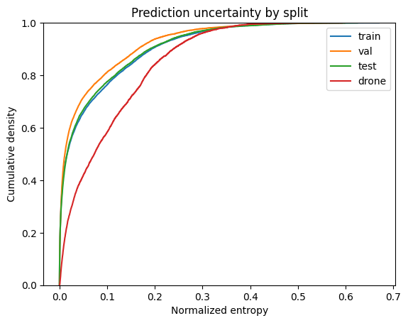
The VOC splits cluster together while the SeaDrone distribution is visibly shifted toward higher entropy — exactly the behavior you would expect from a detector encountering data outside its training distribution.

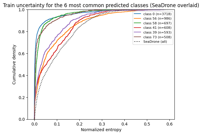
Break uncertainty down per predicted class¶

ClasswiseUncertaintyExtractor groups detections by their predicted class, so you can see which classes the model is most uncertain about rather than only the aggregate. A detection is assigned to every class whose confidence is within a ratio threshold of its top class. The detector predicts across all 80 COCO classes, so to keep the figure legible we plot only the few most frequently predicted classes and overlay the SeaDrone distribution for reference.

TOP_K_CLASSES = 6

uncertainty_by_class = ClasswiseUncertaintyExtractor(scores, preds_type="logits", normalize=True, threshold=0.99)
Hc_train = uncertainty_by_class(trainset)

# The most frequently predicted classes -- best sampled, so their curves are the most reliable
top_classes = sorted(Hc_train, key=lambda cl: len(Hc_train[cl]), reverse=True)[:TOP_K_CLASSES]

plt.figure()
for cl in top_classes:
    plt.ecdf(Hc_train[cl].flatten(), label=f"class {cl} (n={len(Hc_train[cl])})")
plt.ecdf(h_drone.flatten(), linestyle=":", color="k", label="SeaDrone (all)")
plt.xlabel("Normalized entropy")
plt.ylabel("Cumulative density")
plt.title(f"Train uncertainty for the {TOP_K_CLASSES} most common predicted classes (SeaDrone overlaid)")
plt.legend(fontsize=8)
plt.show()

Detect drift with Wasserstein distance¶

Eyeballing ECDFs is useful, but you want an automated decision. DriftWasserstein measures the Wasserstein distance between the reference and incoming uncertainty distributions and flags drift when that distance grows beyond a calibrated baseline.

Unlike most detectors, DriftWasserstein takes two in-distribution references in fit(): a training set and a validation set. The train-vs-validation distance defines the normal amount of variation between two same-distribution samples, so the detector only alarms when incoming data is more different from training than validation was. This calibration is what lets it ignore benign sampling noise.

drift_detector = DriftWasserstein().fit(np.asarray(h_train), np.asarray(h_val))

Now predict on the held-out in-distribution slice (expected: no drift) and on the SeaDrone data (expected: drift). The distance field reports the mean per-feature ratio against the baseline; values above the detector’s ratio_threshold indicate drift.

result_test = drift_detector.predict(np.asarray(h_test))
print(f"VOC held-out -> drift: {result_test.drifted}  (ratio: {result_test.distance:.2f})")

result_drone = drift_detector.predict(np.asarray(h_drone))
print(f"SeaDrone     -> drift: {result_drone.drifted}  (ratio: {result_drone.distance:.2f})")

VOC held-out -> drift: False  (ratio: 0.20)
SeaDrone     -> drift: True  (ratio: 3.43)

The held-out VOC slice stays within the calibrated baseline (no drift), while the SeaDrone data exceeds it (drift detected). The detector turned the visual gap you saw in the ECDF into an automated, label-free alert.

Conclusion¶

In this tutorial you used a deployed detector’s own prediction uncertainty as a drift signal. You decoded raw YOLOv8 output into per-detection class scores, summarized each detection’s confidence as normalized entropy, and used a validation-calibrated DriftWasserstein detector to distinguish benign variation (a held-out VOC slice) from genuine shift (SeaDrone imagery).

Key takeaways:

• Prediction uncertainty is a label-free drift feature — no operational ground truth required

• A postprocess_fn adapts any model’s raw output into the (instances, classes) shape DataEval consumes

• DriftWasserstein calibrates against a validation set, so it alarms on real shift rather than sampling noise

• Per-class breakdowns reveal which classes drive the uncertainty, not just the aggregate

What’s next¶

• Compare this approach with feature-based drift in the monitor shift tutorial

• Read about the taxonomy of shift and when uncertainty-based detection is and isn’t the right tool

• Explore DataEval’s API reference for the full set of drift detectors

Related how-to guides¶

• Detect uncertainty drift with a MAITE model

• Encode a dataset with an ONNX model

• Configure global DataEval defaults

On your own¶

Once you are comfortable with the workflow, adapt it to your own deployed model:

• Swap the model: any classifier or detector works — supply a postprocess_fn for its output format

• Swap the operational data: point the drone split at your real incoming data stream

• Tune sensitivity: adjust DriftWasserstein(ratio_threshold=...) to trade off false alarms against missed drift